6. Linearizing a Non-Linear Relationship
6.1 Introduction
The method of linear regression discussed in Chapter 5 provides a powerful tool for extracting information from data when there is a linear relationships between the variables measured. However, in many cases, the relationship between the experimental variables is not linear. As we will see in the next section, a straightforward graph of such a nonlinear relationship does not tell us very much. It is also more difficult to determine the “best fit” to a nonlinear graph. This chapter will introduce you to methods for creating a linear graph of quantities that we expect to be related nonlinearly. If you can artificially create a linear graph, you can use linear regression to extract information about the relationship that would otherwise be hard to obtain.
6.2 An Example of Linearization
Imagine an experiment where we want to determine an object’s acceleration as it slides from rest down a nearly frictionless incline by measuring its displacement as a function of time. The object should experience a constant acceleration along the incline with a magnitude $a = g\ sin\theta$, where $\theta$ is the angle the incline makes with the horizontal. If we define the z-axis to point down along the incline, then theoretical displacement $d$ of the object as a funciton of the time $t$ since its release is
\begin{equation} d = z - z_0 = \frac{1}{2}at^2, \tag{6.1} \end{equation}where $z_0$ is the starting position.
If we made a graph of $d$ vs. $t$, we would expect a parabola as shown in Figure 6.1. However, it is difficult to distinguish a graph of a $d \propto t^2$ relationship from one showing $d \propto t^3$ or $d \propto t^4$ or other relationships. Since there are a large number of relationships between $d$ and $t$ that could produce similar-looking curves, it is difficult to verify by just looking at the graph that our assumption that the object has constant acceleration is reasonable. In addition, there is no simple way to compute the value of $a$ from this graph.
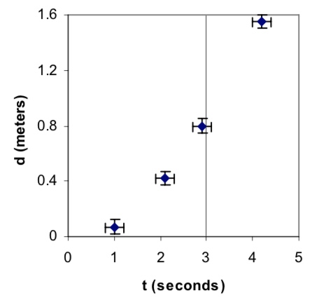 Figure 6.1: Plot of $d$ vs. $t$.
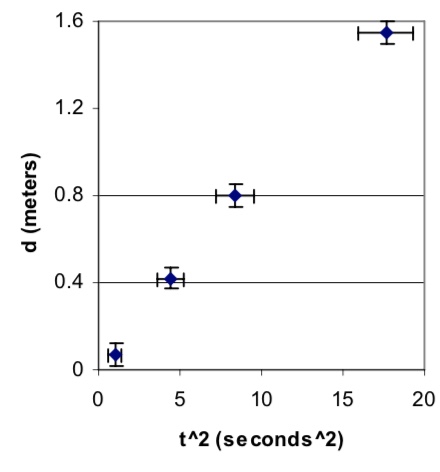
We can address both of these problems by plotting $d$ vs. $t^2$, instead of $t$, as shown in Figure 6.2. In this case, if the object’s acceleration really is constant, then the graph will be a straight line, and if the object’s acceleration is not constant, the graph will be curved. Therefore, a glance at the graph helps us check whether our basic assumption is correct. If the graph does turn out to be a straight line, then the slope of such a graph, whose value and uncertainty can be easily determined using linear regression, will be $a/2$, making it easy to determine the value and uncertainty of $a$. In this case, we expect the intercept to be in agreement with zero when its uncertainty is taken into account. Note that we need to calculate the uncertainty in $t^2$ to draw the horizontal uncertainty bars in Figure 6.2. We get
\begin{equation} U_{t^2} = \sqrt{\left(\frac{\partial (t^2)}{\partial t} U_t\right)^2} = 2t \cdot U_t, \tag{6.2} \end{equation}by using equation 3.1.
For this example, there are other ways to get a linear graph. If we plotted, $\sqrt{d}$ vs. t, the slope should be $\sqrt{a/2}$, since
\begin{equation} \sqrt{d} = \left(\sqrt{a/2}\right) t. \tag{6.3} \end{equation}Alternatively, taking the base-ten logarithm of both sides of equation 6.1 gives
\begin{equation} \log d = z - z_0 = log\left(\frac{1}{2}at^2\right) = log\left(\frac{1}{2}a\right) + 2 \log t. \tag{6.4} \end{equation}If we were to plot $\log d$ vs. $\log t$, then we should get a straight line with slope consistent with 2 and an intercept of $\log \left(a / 2\right)$. This approach would be useful if you wanted to test if $d$ depends on $t^2$ or some other power of $t$, since the power of $t$ is a fit parameter. Note that we would still have to propagated uncertainies to perform the linear regressions, to make the plots, and to find the uncertainty of $a$.
6.3 General Approach to Linearization
It is often, but not always, possible to make a linear graph from measurements. Here are the steps to follow:
- Find a theoretical relation between the two quantities measured.
- Find a function of one variable that when plotted against the other variable (or a function of that second variable) will yield a straight line if the hypothetical relationship is true.
- Make a graph of the variables determined in step 2 using your experimental data to make sure that the plotted quantities lie on a roughly straight line. (If not, try to determine whether your theoretical relation is incorrect or there is some error in your measurements and/or calculations.)
- Compute the uncertainties in the plotted quantities (if different from the measured quantities) using the method described in Chapter 3.
- Use Python to find the slope and intercept of the best fit line and their uncertainties.
- Use the equation found in step 2 to interpret the slope and intercept. You may have to propagate their uncertainties.
6.4 Two Frequently-Used Examples
There are two particular examples that come up so frequently that they merit specific mention.
6.4.1 Exponential Relationships
Many processes, like the voltage across a capacitor as is discharges through a resistor, have an exponential dependence. The general form of an exponential law is
\begin{equation} z = Ce^{Dx}, \tag{6.4} \end{equation}where $D$ can be positive or negative. Taking the natural logarithm of both sides of equation 6.4 gives
\begin{equation} \ln z = \ln C + Dx. \tag{6.5} \end{equation}If we plot $\ln z$ vs. $x$, then comparing with $y = mx + b$ (with $y = \ln z$) the slope should be $D$ and the intercept should be $\ln C$. Don't forget to propagate uncertainties correctly (see Ch. 3). The uncertainty of $\ln z$ isn't the same as the uncertainty of $z$. Also, the uncertainty of $C$ isn't the same as the uncertainty of the intercept.
6.4.2 Power Laws
Another common type of physical relationship is a power law, which is of the form
\begin{equation} y = kx^n, \tag{6.6} \end{equation}where $k$ and $n$ are constants. For example the period of a mass on a spring depends on the square root (1/2 power) of the mass. Taking the base-10 logarithm of equation 6.6 gives
\begin{equation} \log y = \log k + n\log x. \tag{6.7} \end{equation}If we plot $\log y$ vs. $\log x$, the slope should be $n$ and the intercept should be $\log k$. Don't forget to propagate uncertainties correctly (see Ch. 3). The uncertainty of $\log x$ and $\log y$ aren't the same as the uncertainties of $x$ and $y$. Also, the uncertainty of $k$ isn't the same as the uncertainty of the intercept.
6.5 Exercises
6.1 For the hypothetical experiment in section 6.2, suppose that the acceleration $a$ is measured for various angles $\theta$.
(a) What would you plot in order to get a linear graph?
(b) How would the measured graviational acceleartion $g$ be related to the slope $m$ of the best fit line?
(c) If the uncertainty of the slope is $U_m$, what is the uncertainty of the measured graviational acceleartion?
6.2 For section 6.4.1, work out how to propagate the uncertainties.
(a) What is the uncertainty of $\ln z$?
(b) Suppose that linear regression gives values for the slope ($m$), intercept ($b$), and their uncertainties ($U_m$ and $U_b$). What are $C$, $D$, and their uncertainties?
6.3 For section 6.4.2, work out how to propagate the uncertainties.
(a) What is the uncertainty of $\log y$? (The expression for $\log x$ will be similar.)
(b) Suppose that linear regression gives values for the slope ($m$), intercept ($b$), and their uncertainties ($U_m$ and $U_b$). What are $k$, $n$, and their uncertainties?
6.4 The data for the number of bacteria as a function of time in the table below is expected to reflect an exponentially relationship, $N(t) = N_0 e^{\beta t}$.
| time $t$ (min) | Number of bacteria $N$ |
|---|---|
| 10 | 149,000 ± 15,000 |
| 20 | 215,000 ± 20,000 |
| 30 | 335,000 ± 35,000 |
| 40 | 477,000 ± 45,000 |
| 50 | 769,000 ± 75,000 |
(a) Using Python, make a linearized plot of the data by taking a natural logarithm of the number of bacteria. Include error bars. Be sure to propagate the uncertainty in the number of bacteria at each time (see chapter 3).
(b) Use Python to perform a linear fit, finding the slope, the intercept, and their uncertainties.
(c) Find the values of $\beta$ and $N_0$ that best fit the data and their uncertainties.
6.5 The table below gives the orbital periods $T$ (in years) of the planets known to Newton as a function of their mean distance $R$ from the sun in AUs (where 1 AU = the earth’s mean orbital radius). The period and distance are related by a power-law of the form $T=kR^n$.
| Planet | Distance (AU) | Period (yr) |
|---|---|---|
| Mercury | 0.39 | 0.24 |
| Venus | 0.72 | 0.62 |
| Earth | 1.00 | 1.00 |
| Mars | 1.52 | 1.88 |
| Jupiter | 5.20 | 11.86 |
| Saturn | 9.54 | 29.46 |
(a) Using Python, make a linearized plot of the data by taking the base-10 logarithm of the distance and period. Also, use Python to find the slope and the intercept of the best-fit line.
(b) What does the fit suggest are the likely values of $k$ and $n$?