Linear Regression in plain Python
In linear regression we want to model the relationship between a scalar dependent variable $y$ and one or more independent (predictor) variables $\boldsymbol{x}$.
Given:
- Dataset $D = \{(\pmb{x}^{(1)}, y^{(1)}), ..., (\pmb{x}^{(m)}, y^{(m)})\}$
- With $\pmb{x}^{(i)}$ being a $d-$dimensional vector $\pmb{x}^{(i)} = (x^{(i)}_1, ..., x^{(i)}_d)$ and
- $y^{(i)}$ being a scalar target variable
Assumptions:
- We assume that dataset was produced by some unknown function $f$ which maps features $\pmb{x}$ to labels $y$
- We further assume that the labels $y^{(i)}$ are noisy
- In other words: the labels have been produced by adding some noise $\epsilon$ to the true function value: $y^{(i)} = f(\pmb{x}^{(i)}) + \epsilon$
Model:
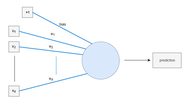
The linear regression model can be interpreted as a very simple neural network:
- It has a real-valued weight vector $\pmb{w}= (w_{1}, ..., w_{d})$
- It has a real-valued bias $b$
- It uses the identity function as its activation function
- Note: in most books the parameter vector $\pmb{w}$ is denoted in a more general form, namely as $\pmb{\theta}$
Approach:
Our goal is to learn the underlying function $f$ such that we can predict function values at new input locations. In linear regression, we model $f$ using a linear combination of the input features:
Training
A linear regression is typically trained using the (mean) squared error (MSE) as a loss function. This computes a least squares solution. The mean squared error minimizes the sum of squared residuals (= difference between true label $y$ and the model prediction $\hat{y}$):
$J(\boldsymbol{w},b) = \frac{1}{m} \sum_{i=1}^m \Big(\hat{y}^{(i)} - y^{(i)} \Big)^2$
Why do we use the squared error as a loss function? In short, using the MSE corresponds to computing a maximum likelihood solution to our problem. For a more detailed explanation look here.
With the MSE at hand a linear regression model can be trained using either
a) gradient descent or
b) the normal equation (closed-form solution): $\boldsymbol{w} = (\boldsymbol{X}^T \boldsymbol{X})^{-1} \boldsymbol{X}^T \boldsymbol{y}$
where $\boldsymbol{X}$ is a matrix of shape $(m, n_{features})$ that holds all training examples.
The normal equation requires computing the inverse of $\boldsymbol{X}^T \boldsymbol{X}$. The computational complexity of this operation lies between $O(n_{features}^{2.4}$) and $O(n_{features}^3$) (depending on the implementation).
Therefore, if the number of features in the training set is large, the normal equation will get very slow.
The training procedure of a linear regression model has different steps. In the beginning (step 0) the model parameters are initialized. The other steps (see below) are repeated for a specified number of training iterations or until the parameters have converged.
Step 0:
Initialize the weight vector and bias with zeros (or small random values)
OR
Compute the parameters directly using the normal equation
Step 1: (Only needed when training with gradient descent)
Compute a linear combination of the input features and weights. This can be done in one step for all training examples, using vectorization and broadcasting: $\boldsymbol{\hat{y}} = \boldsymbol{X} \cdot \boldsymbol{w} + b $
where $\boldsymbol{X}$ is a matrix of shape $(m, n_{features})$ that holds all training examples, and $\cdot$ denotes the dot product.
Step 2: (Only needed when training with gradient descent)
Compute the cost (mean squared error) over the training set:
$J(\boldsymbol{w},b) = \frac{1}{m} \sum_{i=1}^m \Big(\hat{y}^{(i)} - y^{(i)} \Big)^2$
Step 3: (Only needed when training with gradient descent)
Compute the partial derivatives of the cost function with respect to each parameter:
$ \frac{\partial J}{\partial w_j} = \frac{2}{m}\sum_{i=1}^m \Big( \hat{y}^{(i)} - y^{(i)} \Big) x^{(i)}_j$
$ \frac{\partial J}{\partial b} = \frac{2}{m}\sum_{i=1}^m \Big( \hat{y}^{(i)} - y^{(i)} \Big)$
The gradient containing all partial derivatives can then be computed as follows:
$\nabla_{\boldsymbol{w}} J = \frac{2}{m} \boldsymbol{X}^T \cdot \big(\boldsymbol{\hat{y}} - \boldsymbol{y} \big)$
$\nabla_{\boldsymbol{b}} J = \frac{2}{m} \big(\boldsymbol{\hat{y}} - \boldsymbol{y} \big)$
Step 4: (Only needed when training with gradient descent)
Update the weight vector and bias:
$\boldsymbol{w} = \boldsymbol{w} - \eta \, \nabla_w J$
$b = b - \eta \, \nabla_b J$
where $\eta$ is the learning rate.
import numpy as np
import matplotlib.pyplot as plt
from sklearn.model_selection import train_test_split

np.random.seed(123)
Dataset
# We will use a simple training set
X = 2 * np.random.rand(500, 1)
y = 5 + 3 * X + np.random.randn(500, 1)

fig = plt.figure(figsize=(8,6))
plt.scatter(X, y)
plt.title("Dataset")
plt.xlabel("First feature")
plt.ylabel("Second feature")
plt.show()

# Split the data into a training and test set
X_train, X_test, y_train, y_test = train_test_split(X, y)

print(f'Shape X_train: {X_train.shape}')
print(f'Shape y_train: {y_train.shape}')
print(f'Shape X_test: {X_test.shape}')
print(f'Shape y_test: {y_test.shape}')
Shape X_train: (375, 1)
Shape y_train: (375, 1)
Shape X_test: (125, 1)
Shape y_test: (125, 1)
Linear regression class
class LinearRegression:

    def __init__(self):
        pass

    def train_gradient_descent(self, X, y, learning_rate=0.01, n_iters=100):
        """
        Trains a linear regression model using gradient descent
        """
        # Step 0: Initialize the parameters
        n_samples, n_features = X.shape
        self.weights = np.zeros(shape=(n_features,1))
        self.bias = 0
        costs = []

        for i in range(n_iters):
            # Step 1: Compute a linear combination of the input features and weights
            y_predict = np.dot(X, self.weights) + self.bias

            # Step 2: Compute cost over training set
            cost = (1 / n_samples) * np.sum((y_predict - y)**2)
            costs.append(cost)

            if i % 100 == 0:
                print(f"Cost at iteration {i}: {cost}")

            # Step 3: Compute the gradients
            dJ_dw = (2 / n_samples) * np.dot(X.T, (y_predict - y))
            dJ_db = (2 / n_samples) * np.sum((y_predict - y))

            # Step 4: Update the parameters
            self.weights = self.weights - learning_rate * dJ_dw
            self.bias = self.bias - learning_rate * dJ_db

        return self.weights, self.bias, costs

    def train_normal_equation(self, X, y):
        """
        Trains a linear regression model using the normal equation
        """
        self.weights = np.dot(np.dot(np.linalg.inv(np.dot(X.T, X)), X.T), y)
        self.bias = 0

        return self.weights, self.bias

    def predict(self, X):
        return np.dot(X, self.weights) + self.bias
Training with gradient descent
regressor = LinearRegression()
w_trained, b_trained, costs = regressor.train_gradient_descent(X_train, y_train, learning_rate=0.005, n_iters=600)

fig = plt.figure(figsize=(8,6))
plt.plot(np.arange(600), costs)
plt.title("Development of cost during training")
plt.xlabel("Number of iterations")
plt.ylabel("Cost")
plt.show()
Cost at iteration 0: 66.45256981003433
Cost at iteration 100: 2.2084346146095934
Cost at iteration 200: 1.2797812854182806
Cost at iteration 300: 1.2042189195356685
Cost at iteration 400: 1.1564867816573
Cost at iteration 500: 1.121391041394467

Testing (gradient descent model)
n_samples, _ = X_train.shape
n_samples_test, _ = X_test.shape

y_p_train = regressor.predict(X_train)
y_p_test = regressor.predict(X_test)

error_train =  (1 / n_samples) * np.sum((y_p_train - y_train) ** 2)
error_test =  (1 / n_samples_test) * np.sum((y_p_test - y_test) ** 2)

print(f"Error on training set: {np.round(error_train, 4)}")
print(f"Error on test set: {np.round(error_test)}")
Error on training set: 1.0955
Error on test set: 1.0
Training with normal equation
# To compute the parameters using the normal equation, we add a bias value of 1 to each input example
X_b_train = np.c_[np.ones((n_samples)), X_train]
X_b_test = np.c_[np.ones((n_samples_test)), X_test]

reg_normal = LinearRegression()
w_trained = reg_normal.train_normal_equation(X_b_train, y_train)
Testing (normal equation model)
y_p_train = reg_normal.predict(X_b_train)
y_p_test = reg_normal.predict(X_b_test)

error_train =  (1 / n_samples) * np.sum((y_p_train - y_train) ** 2)
error_test =  (1 / n_samples_test) * np.sum((y_p_test - y_test) ** 2)

print(f"Error on training set: {np.round(error_train, 4)}")
print(f"Error on test set: {np.round(error_test, 4)}")
Error on training set: 1.0228
Error on test set: 1.0432
Visualize test predictions
# Plot the test predictions

fig = plt.figure(figsize=(8,6))
plt.title("Dataset in blue, predictions for test set in orange")
plt.scatter(X_train, y_train)
plt.scatter(X_test, y_p_test)
plt.xlabel("First feature")
plt.ylabel("Second feature")
plt.show()
