Predicting Patient Outcomes of Artificial Heart Implant
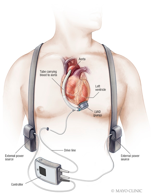
The artificial heart, VAD (ventricular assist device), is an implantable electromechanical device used to partially replace the function of a heart. It is the last therapeutic treatment for people in end-stage heart failure. VADs were expected to extend patients lives for several years. However, many patients who received VADs died shortly after the implant.
In this project, I mine previous VAD recipients' clinical records and outcomes, and build machine learning models that can help physicians to predict the likely outcome of each implant.
<img src="https://www.mayoclinic.org/-/media/kcms/gbs/patient-consumer/images/2013/11/15/17/38/my01077_my00361_im04277_mcdc7_lvadthu_jpg.jpg", width=250>
Data Science Problem, Goal and Prior Work:
I used the INTERMACS dataset for this project. This dataset includes 23,787 patients' clinical data relevant to mechanical circulatory support devices (VAD is one kind of such devices) from initial hospitalization through post-implant follow-up evaluations. Their pre-implant clinical conditions served as starting places for my feature engineering, and the time interval between their implant and death/explant is the training labels.
Comparable previous works on VAD implant prognostics using INTERMACS data most often used linear regression or Bayesian models. The accuracy of one-year mortality predictions is 83% to 84.5%.
** Table of Content: **
-
- Prognostic Fairness
- Patient Clustering
- Deep Learning
# utility
import pandas as pd
import numpy as np
import json
from collections import Counter
def pprintDict(d):
'''pretty print dictionary'''
print(json.dumps(d, sort_keys=True, indent=4))
import warnings
warnings.simplefilter('ignore')
# stats and machine learning
import math
import random as rand
import scipy.stats as stats
import scipy.sparse as sp
from sklearn import dummy, preprocessing, feature_selection, feature_extraction, metrics, model_selection
from sklearn import tree, multiclass, svm, ensemble, gaussian_process, neighbors
from sklearn.linear_model import LinearRegression
# from point import Point
from imblearn.combine import SMOTETomek # https://github.com/scikit-learn-contrib/imbalanced-learn
# visualization
import matplotlib
import matplotlib.pyplot as plt
plt.style.use('ggplot')
import seaborn as sns
sns.set_style("white")
sns.set_palette("PuBuGn_d")
from matplotlib.ticker import FuncFormatter
%matplotlib inline
1 - Data Preparation
1.1 - Consolidating INTERMACS databases
I elicited data of the patients who have received VAD implants and have died or explanted. Please see dataprep.py for the implementation of this part.
- Combine four INTERMACS databases. Here I took all columns as objects (str) for the moment.
patient_INTERMACS_Data_Dictionary.csvdevice_INTERMACS_Data_Dictionary.csvfollowup_INTERMACS_Data_Dictionary.csv
- Elicitating patients who eventually received an artificial heart;
- Focusing on first-time implant patients;
- Seperating pre-implant and post-implant variables;
- Set INT_DEAD (integer) as label.
from dataprep import feature_dict, import_and_join
# Import Data
feature_dict = feature_dict()
df, input_col, outcome_col, idx_col = import_and_join(feature_dict)
df.head()
Integrated and imported 551 input columns, 118 output columns and 5821 observations.
| PATIENT_ID | CC_ADVANCED_AGE_M | CC2_ADVANCED_AGE_M | CC_ALLOSENSITIZATION_M | CC2_ALLOSENSITIZATION_M | CC_CHRONIC_COAGULOPATHY | CC2_CHRONIC_COAGULOPATHY | CC_CHRONIC_INF_CONCERNS_M | CC2_CHRONIC_INF_CONCERNS_M | CC_CHRONIC_RENAL_DISEASE_M | ... | OP4EXPL | OP4EXPREA | OP4INTD | OP4INTR | OP4INTT | OP4REC | OP4TXPL | TRANSFER_CARE | TREC_PT | TXPL_PT | |
|---|---|---|---|---|---|---|---|---|---|---|---|---|---|---|---|---|---|---|---|---|---|
| 2 | 12 | Missing | No | Missing | No | Missing | Missing | Missing | No | Missing | ... | 0.0 | nan | 7.162364730299999 | 7.162364730299999 | 7.162364730299999 | 0.0 | 0.0 | nan | 0.0 | 0.0 |
| 3 | 12 | No | No | No | No | No | No | No | No | No | ... | nan | nan | nan | nan | nan | nan | nan | nan | nan | nan |
| 4 | 12 | No | No | No | No | No | No | No | No | No | ... | nan | nan | nan | nan | nan | nan | nan | nan | nan | nan |
| 5 | 12 | No | No | No | No | No | No | Yes | Yes | No | ... | nan | nan | nan | nan | nan | nan | nan | nan | nan | nan |
| 6 | 13 | Missing | No | Missing | No | Missing | Missing | Missing | No | Missing | ... | nan | nan | nan | nan | nan | nan | nan | nan | 0.0 | 0.0 |
5 rows × 672 columns
pprintDict(feature_dict['LVEF'])
{
"FORMAT": "ISF_LVEF.",
"FORMAT_VALUE": {
"1": "> 50 (normal)",
"2": "40-49 (mild)",
"3": "30-39 (moderate)",
"4": "20-29 (moderate/severe)",
"5": "Not Recorded or Not Documented",
"6": "< 20 (severe)",
"998": "~Unknown~"
},
"LABEL": "LVEF",
"TYPE": "Num"
}
1.2 - Correcting Data Types and Value Mappings
The feature dictionary shows the current encoding of the dataset is largely impropriate.
Many numeric attributes in the data do not represent numeric meanings or distances, and same as nominal attributes.
Missing values are also often represented with strings, numbers and others. When importing the databases, we have dealt with common NaN encodings but not others ('998', '-', 'Not Done', 'Unknown', '~Unknown~', etc.)
Even worse is that columns with name that ends with
_Mhave already been mapped to a different set of value during data collection, require us to "de-code" them back.For exmaple, the "LVEF" (left ventricular ejection fraction, the percentage number of total amount of blood in the left ventricle is pumped out with each heartbeat) attribute is represented as below. Encoding "Not Recorded or Not Documented" as "5" doesn't really make sense. Similarly dangerous is to interpret '998' as numeric instead of NaN.
| value encoding in the raw data | actual LVEF value |
|---|---|
| 1 | > 50 (normal) |
| 2 | 40-49 (mild) |
| 3 | 30-39 (moderate) |
| 4 | 20-29 (moderate/severe) |
| 5 | Not Recorded or Not Documented |
| 6 | < 20 (severe) |
| 998 | ~Unknown~ |
To correct these messy data encodings, I used two approach.
- I extracted mappings from the feature dictionary and transformed the data accordingly. For example, I mapped 'blood_type' (numeric) attribute to nominal and NANs based on the feature dict annotation:
blood_type = {1: 'O', 2: 'A', 3: 'B', 4: 'AB', 998: '-'}
- I manually created some mapping dictionaries to encode some attributes in a more meaningful way. Please see
dataprep.pyfor the implementation of this procedure. For example, I translated 'time_card_dgn' (time of cardiology diagnosis) from nominal to numeric values.
time_card_dgn = {'< 1 month': 0, '1 month - 1 year': 1, '1-2 years': 12, '> 2 years': 24, '-': np.nan}
def init_df_encoding(df, feature_dict, verbose = False):
'''
Encoding the NANs and "Other"s for df based on feature_dict
@param: Raw dataset (df) and feature dictionary (dict) curated by dataprep.py
Every item in feature_dict has key ['FORMAT_VALUE'] who
@output: Encoded df (df)
'''
nan_encodings = ['-',
'Not Recorded or Not Documented',
'Unknown', '~Unknown~',
'Missing',
'MISSING',
'Not Done',
'Not Applicable',
'N/A',
'Unspecified']
other_encodings = ['Other,Specify',
'Other,specify',
'Other, specify',
'~Other, specify~',
'Other']
for col in df.columns:
# if FORMAT_VALUE has value, need additional NaA decoding
if isinstance(feature_dict[col]['FORMAT_VALUE'], dict):
# for each column, find the values (i.e. 998, '-', etc.) that represent nan_encodings
nan_this_col = set([v for k, v in feature_dict[col]['FORMAT_VALUE'].items() if v in nan_encodings]+ [k for k, v in feature_dict[col]['FORMAT_VALUE'].items() if v in nan_encodings])
# replace these values with NaNs
nan_this_col = {key: None for key in nan_this_col}
df[col] = df[col].replace(nan_this_col)
# replace "nan" (default NaN representation in INTERMACS) with None
df[col] = df[col].replace({'nan': None})
if col not in ['NYHA']:
df[col] = df[col].apply(pd.to_numeric, errors='ignore')
if verbose:
print('datatype overview:')
for key, value in Counter(df.dtypes.values).items():
print('>>>', key, value)
return df
df = init_df_encoding(df, feature_dict, verbose = True)
datatype overview: >>> float64 224 >>> object 440 >>> int64 8
1.3 - Train-Validation-Test Split
def df_split(df, test_size = 0.1, validation_size = 0.2, verbose = True):
'''
Drop the patient cases whose INT_DEAD value (label) is missing (these are likely to be patients who have been explanted or are still alive to date)
and split the data into train, validation and test sets.
@param: dataset (dataframe) with a 'INT_DEAD' column
@output: X_train, X_valid, X_test, y_train, y_valid, y_test, Xa, ya (dataframes)
Xa and ya are combinations of train and validation sets, used for building the model for final testing
'''
df = df[df['INT_DEAD'].notnull()]
Xa, X_test, ya, y_test = model_selection.train_test_split(df[input_col], df['INT_DEAD'], test_size = test_size, random_state=0)
X_train, X_valid, y_train, y_valid = model_selection.train_test_split(Xa, ya, test_size = validation_size, random_state=0)
X_train.reset_index(drop = True, inplace = True)
X_valid.reset_index(drop = True, inplace = True)
X_test.reset_index(drop = True, inplace = True)
if verbose:
assert (len(X_train.columns) == len(X_valid.columns) and len(X_train.columns) == len(X_test.columns))
assert (len(X_train) == len(y_train) and len(X_valid) == len(y_valid) and len(X_test) == len(y_test))
print('%d feature columns.' % len(X_train.columns))
print('%d instances in the train set; %d in validation; %d in test.'%(len(X_train), len(X_valid), len(X_test)))
print('# of missing value:', X_train.isnull().sum().sum()) # 1521691
print('% of missing value:', "{0:.2f}%".format(X_train.isnull().sum().sum() * 100 / (len(X_train) * len(X_train.columns))))
return X_train, X_valid, X_test, y_train, y_valid, y_test, Xa, ya
X_train, X_valid, X_test, y_train, y_valid, y_test, Xa, ya = df_split(df, 0.1, 0.2)
551 feature columns. 4190 instances in the train set; 1048 in validation; 583 in test. # of missing value: 830841 % of missing value: 35.99%
<img src='http://www.clker.com/cliparts/5/8/1/a/12065629301845618631qubodup_16x16px-capable_black_and_white_icons_7.svg.hi.png', width = 30, style="float: left; margin-left:150px; margin-right: 10px"> Shockingly, 36% of the training data is NANs. This is a major issue that I will address in my later data cleaning and modeling.
2 - Problem Setup and Baseline
With the datasets ready, I now build a dummy model to estimate the baseline performance. The basic data processing (i.e. imputation, categorical attribute encoding) and model evaluation functions written in this process will be used in building and evaluating the more sophisticated models as well.
Utility Functions
- Preliminary data processing:
def filling_NAs(df):
"""
fill in missing values in numeric columns with column means
:param df: dataframe
:return: imputed dataframe
"""
fill = preprocessing.Imputer(strategy='mean')
df_imputed = fill.fit_transform(df) # returns ndarray
return pd.DataFrame(df_imputed)
def encoding_trainX(nominal_col):
"""
transform a column of categorical values (in the training data) to numeric;
:param: nominal_col (array)
:returns: encoded column (array),
label encoder (preprocessing.LabelEncoder.classes_ in sklearn)
"""
col = nominal_col.fillna('0')
le = preprocessing.LabelEncoder()
le.fit(col)
encoded_col = le.transform(col)
return encoded_col, le.classes_
def encoding_trainX_wrapper(X):
'''
transform categorical values in the df to numeric
and store the property of the encoder
:param: X (df)
:returns: encoded X (df) and label encoder (dict of col_name - preprocessing.LabelEncoder pairs)
'''
encoder_dict = {}
for col_name in X.select_dtypes(include=['object']):
coli, lei = encoding_trainX(X[col_name])
X.loc[:,col_name] = coli
encoder_dict[col_name] = lei
return X, encoder_dict
def dummy_prep_trainX(X):
'''
preprocess features in training data
wrapping functions of encoding labels and filling in NAs
@param: X (df);
encoder_dict (dict of col_name - preprocessing.LabelEncoder pairs)
'''
X, encoder_dict = encoding_trainX_wrapper(X)
X = filling_NAs(X)
return X, encoder_dict
def encoding_testX(Xtest, encoder_dict):
'''
transform categorical values in the df to numeric;
@param: X (df) and encoder_dict (dict of col_name - preprocessing.LabelEncoder pairs)
'''
for col_name in list(encoder_dict):
# for col_name in Xtest.select_dtypes(include=['object']):
encoderi = preprocessing.LabelEncoder()
encoderi.classes_ = encoder_dict[col_name]
Xtest.loc[:,col_name] = encoderi.transform(Xtest[col_name])
return Xtest
def dummy_prep_testX(X, encoder_dict):
'''
preprocess new incoming features - encode labels and fill in NAs
@param: X (df), label_encoder (preprocessing.LabelEncoder in sklearn)
@returns: encoded X (df)
'''
# first, use the encoders created with Xtrain to encode Xtest
X = encoding_testX(X, encoder_dict)
# then encode other nominal columns
X, _ = encoding_trainX_wrapper(X)
X = filling_NAs(X)
return X
- Regression model evaluation
def standard_eval(ytest, yhat, graph_title = 'untitled', graph = True):
'''
plot *regression* targets and results
:param: ytest (Series), yhat (Series), graph_title(str).
'''
df = pd.concat([ytest, pd.Series(yhat)], axis=1, ignore_index=True)
df.columns = ['True_Value', 'Prediction']
df = df.fillna(0).sort_values('True_Value').reset_index(drop=True) # remove empty predictions [~df['y_true'].isnull()]
if graph:
# plot y_true vs. y_pred
tidy = (
df.stack() # pull the columns into row variables
.to_frame() # convert the resulting Series to a DataFrame
.reset_index() # pull the resulting MultiIndex into the columns
.rename(columns={'level_0': 'index', 'level_1': 'target', 0: 'INT_DEAD (mo)'}) # rename the unnamed column
)
sns.lmplot(x = 'index' , y = 'INT_DEAD (mo)', hue = 'target', data = tidy, fit_reg=False,
size = 6,
markers = ['x', '1'], palette = dict(True_Value="#9b59b6", Prediction="#3498db"))
plt.title(graph_title, fontsize = 14)
plt.xlabel('observations')
plt.ylabel('(months)')
plt.ylim(0, min(110, max(df['True_Value'])))
plt.savefig('plot/%s.eps' %graph_title, format='eps', dpi=300)
plt.show()
# The mean squared error
print(">> MSE: %.2f" % metrics.mean_squared_error(ytest, yhat))
print(">> MAE: %.2f" % metrics.mean_absolute_error(ytest, yhat))
# Explained variance score: 1 is perfect prediction
print('>> R2: %.2f' % metrics.r2_score(ytest, yhat))
- Set up Model object, parent class of all later machine learning models
class model(object):
"""
model.train() return the model(variable types depends on model)
model.getPerformance() (return the ROC and accuracy in dictionary format)
model.predict(v): pass in a 1xn array and return prediction value
"""
def __init__(self):
self.train
self.predict
self._eval
def __repr__ (self):
return ((self.name,self.performance))
def __hash__(self):
return hash((self.name))
def __eq__(self,other):
return(isinstance(other,model)and(self.name==other.name) \
and (self.data==other.data))
def train(self):
pass
def predict(self, Xtest):
pass
def _eval(self, Xtest, ytest, graph_title):
pass
Baseline Regression Models
Build a (dead) simple linear regressor to estimate baseline performance:
class DummyLinReg(model):
def __init__(self):
self.weights = []
self.le = None # label encoder for categorical data (dictionary of encoders)
model.__init__(self)
def train(self, X, y):
"""
Train a linear regression model
:parma X: n (# of observations) x p (# of features) design matrix
:param y: response vector of length n
:return weights: weight vector of length p
"""
X, self.le = dummy_prep_trainX(X)
regr = LinearRegression(fit_intercept=False)
regr.fit(X, y)
self.model = regr
self.weights = regr.coef_
def predict(self, X):
yhat = np.dot(X, self.weights)
return yhat
def _eval(self, Xtest, ytest, graph_title):
Xtest = dummy_prep_testX(Xtest, self.le)
yhat = self.predict(Xtest)
standard_eval(ytest, yhat, graph_title)
# baseline model
baselineLR = DummyLinReg()
baselineLR.train(X_train, y_train)
baselineLR._eval(X_train, y_train, 'Baseline Linear Regression | Test on Training Set')
baselineLR._eval(X_valid, y_valid, 'Baseline Linear Regression | Test on Validation Set')

>> MSE: 64.26 >> MAE: 4.25 >> R2: 0.69

>> MSE: 607168291162.13 >> MAE: 42345.39 >> R2: -2721473088.80
The disparity between the Linear Regressor's train/validation set performances suggests that the dummy features are likely to be too many/noisy. Let's instead compute a higher baseline with a median dummy regressor instead.
def dumReg(X_train, y_train, X_valid, y_valid):
X_train, le_dict = dummy_prep_trainX(X_train)
X_valid = dummy_prep_testX(X_valid, le_dict)
Dum = dummy.DummyRegressor(strategy="median")
Dum.fit(X_train, y_train)
print("Performance on training set:")
standard_eval(y_train, Dum.predict(X_train), graph = False)
print("Performance on validation set:")
standard_eval(y_valid, Dum.predict(X_valid), graph = False)
dumReg(X_train, y_train, X_valid, y_valid)
Performance on training set: >> MSE: 242.23 >> MAE: 9.95 >> R2: -0.17 Performance on validation set: >> MSE: 255.95 >> MAE: 9.92 >> R2: -0.15
Best Performing Classifier in Literature
Clinical literature often evaluate models based on clinical endpoints (i.e. survival rate after 30 days, 90 days, 6 month, 1 year, and 2 years postimplant). For performance comparison, I buid classifiers for these end points as well.
def bucket_y(y, bucket_array = [0, 1, 3, 6, 12, 24, np.inf]):
'''
:param: Series of continous numbers
:return: Series of categorical values
'''
y = [str(yi) for yi in pd.cut(y, bucket_array)]
return pd.Series(y)
def clf_standard_eval(ytrue, yhat, verbose = True):
'''
transform regressor predictions into categorical
to evaluate accuracy in terms of endpoint survival (1mo, 3mo, 6mo, 1 yr, 2yr)
@params: ytrue (Series) and yhat (Series)
'''
yhat = bucket_y(yhat, [-np.inf, 1, 3, 6, 12, 24, np.inf])
ytrue = bucket_y(ytrue, [-np.inf, 1, 3, 6, 12, 24, np.inf])
accu = metrics.accuracy_score(ytrue, yhat)
f1 = metrics.f1_score(ytrue, yhat, average = 'weighted')
if verbose:
print('accuracy: {0:.2f}%'.format(accu))
print('F1: {0:.2f}%'.format(f1))
print(metrics.classification_report(ytrue, yhat))
return accu
def dummpyClf(X_train, y_train, X_valid, y_valid):
# transform y from numeric to categorical
y_train = bucket_y(y_train)
y_valid = bucket_y(y_valid)
X_train, selector = dummy_prep_trainX(X_train)
X_valid = dummy_prep_testX(X_valid, selector)
n_classes = len(y_valid.unique())
# multi-class classifier
# clf = multiclass.OneVsRestClassifier(dummy.DummyClassifier(strategy="most_frequent"))
# clf.fit(X_train, y_train)
# y_hat = clf.predict(X_valid)
# print('Validation accuracy: {0:.2f}%'.format(metrics.accuracy_score(y_valid, y_hat) * 100))
for label in sorted(y_valid.unique()):
y_traini = (y_train == label).astype('int') # binary classes
y_validi = (y_valid == label).astype('int')
clf = dummy.DummyClassifier(strategy="stratified")
clf.fit(X_train, y_traini)
y_scores = clf.predict_proba(X_valid)
y_hati = clf.predict(X_valid)
print('Target: %s months survival' % label)
print('>> AUROC: {0:.2f}%'.format(metrics.roc_auc_score(np.array(y_validi),y_hati) * 100 ))
print('>> validation accuracy: {0:.2f}%'.format(metrics.accuracy_score(y_validi, y_hati) * 100))
# plot_roc(clf, X_valid, y_validi)
dummpyClf(X_train, y_train, X_valid, y_valid)
Target: (0.0, 1.0] months survival >> AUROC: 50.88% >> validation accuracy: 66.98% Target: (1.0, 3.0] months survival >> AUROC: 52.15% >> validation accuracy: 72.90% Target: (12.0, 24.0] months survival >> AUROC: 47.87% >> validation accuracy: 69.47% Target: (24.0, inf] months survival >> AUROC: 52.32% >> validation accuracy: 73.76% Target: (3.0, 6.0] months survival >> AUROC: 47.58% >> validation accuracy: 76.72% Target: (6.0, 12.0] months survival >> AUROC: 50.26% >> validation accuracy: 75.19%
Intuitions:
The inherent characteristics of this dataset posed several challenges to machine learning. These characteristics anchored many choices we made in data cleaning and the later modeling process.
- Feature selection. sparse data / missing values, feature redundancy
- 90 days and 6 months fits their Bayesian models relatively poorly
- Explainabile models only
Overview and Transform Prediction targets
Knowing that historically some targets (mortality interval of certain lenght) are more difficult to predict than others, I look into the distribution of these targets. If appropriate, I can potantially transform the targets to make them easier to fit with relatively simple models (i.e. linear models).
min(y_train), max(y_train)
(0.016427442, 100.7330746)
Counter(round(y_train,9) < 1)
Counter({False: 3289, True: 901})
def plot_y_hist(X_train, y_train, to_file = False):
fig, ax = plt.subplots()
ax = y_train.hist(figsize=(12, 4), bins = 110, density = True, color = 'black', edgecolor = 'white')
ax.set_yticklabels(['{:3.2f}%'.format(x*100) for x in ax.get_yticks()])
ax.set_title('INT_DEATH distribution (time interval between surgery and death)')
plt.xlabel('(months)')
if to_file == True:
plt.savefig('plot/viz1.eps', format='eps', dpi=300)
plt.show()
plot_y_hist(X_train, y_train, to_file = True)

def plot_y_log_prob(X_train, y_train, to_file = False):
fig = plt.figure(figsize=(5, 4))
ax = fig.add_subplot(111)
y_train_log = np.log(y_train) # log1p inverse: np.expm1
stats.probplot((y_train_log - np.mean(y_train_log))/np.std(y_train_log),plot=plt)
ax.get_lines()[0].set_markerfacecolor('dimgray')
ax.get_lines()[0].set_alpha(0.1)
ax.get_lines()[0].set_markeredgecolor('black')
ax.get_lines()[1].set_color('orangered')
if to_file == True:
plt.savefig('plot/viz2.eps', format='eps', dpi=300)
plt.show()
plot_y_log_prob(X_train, y_train, to_file = False)

def plot_nyha(X_train, y_train_log, to_file = False):
nyha_fig = plt.figure(figsize=(20, 3))
nyha_fig.suptitle('log(INT_DEATH)', fontsize=14)
pos = 161
for nyha, group in X_train.groupby('NYHA'):
yi = y_train_log[group.index]
ax = nyha_fig.add_subplot(pos)
stats.probplot((yi - np.mean(yi))/np.std(yi),plot=ax)
ax.get_lines()[0].set_markerfacecolor('dimgray')
ax.get_lines()[0].set_alpha(0.3)
ax.get_lines()[0].set_markeredgecolor('black')
ax.get_lines()[1].set_color('orangered')
if nyha == '-':
nyha = 'Unknown'
ax.set_title("NYHA %s -- %d Patients" % (nyha, len(yi)), fontsize = 14)
pos += 1
plt.subplots_adjust(left=0.1, wspace=0.2, top=0.8)
if to_file == True:
plt.savefig('plot/viz3.eps', format='eps', dpi=300)
plt.show()
plot_nyha(X_train, np.log(y_train), to_file = False)

# baseline model
BL = DummyLinReg()
BL.train(X_train, np.log(y_train))
print('Training:')
BL._eval(X_train, np.log(y_train), 'DummyLinReg log(y) | Test on Training Set')
print('Validation:')
BL._eval(X_valid, np.log(y_valid), 'DummyLinReg log(y) | Test on Validation Set')
dumReg(X_train, np.log(y_train), X_valid, np.log(y_valid))
So we will potentially build differet models for this
Dealing with and Utilizing (Lots of) Missing Values:
print('# of missing value:', X_train.isnull().sum().sum()) # 1521691
print('% of missing value:', "{0:.2f}%".format(X_train.isnull().sum().sum() * 100 / (len(X_train) * len(X_train.columns))))
# of missing value: 440477 % of missing value: 19.01%
def plot_na(X):
'''
:param: training data (df)
'''
fig, ax = plt.subplots(1,2, figsize=(12,3))
# plot % of missing value in each column
na_ptg = [ cent/len(X) for cent in X.isnull().sum().values]
sns.distplot(na_ptg, kde=False, bins = 25, ax=ax[0])
xticks = ax[0].get_xticks()
ax[0].set_xticklabels(['{:.0f}%'.format(x * 100) for x in xticks])
ax[0].set_title('% of Missing Value Per Column')
sns.distplot([ptg for ptg in na_ptg if ptg > 0.9], kde=False, bins = 10, ax=ax[1])
xticks = ax[1].get_xticks()
ax[1].set_xticklabels(['{:.0f}%'.format(x * 100) for x in xticks])
ax[1].set_title('% of Missing Value Per Column (close-up)')
plot_na(X_train)

To take a closer look, I used msno.matrix nullity matrix, a data-dense display which quickly visually picks out patterns in data completion. The sparkline at right summarizes the general shape of the data completeness and points out the maximum and minimum rows.
from quilt.data.ResidentMario import missingno_data
import missingno as msno
# Note that msno visualization accommodates up to 50 labelled variables.
# This dataframe exceeds this range thus labels begin to overlap or become unreadable.
# Therefore I divided up the dataframe for closer inspection.
i = 0
for Xi in np.array_split(X_train, 15, axis = 1):
msno.matrix(Xi.sample(100))
plt.savefig('plot/na_pattern_%s.png' % str(i), dpi=300)
i += 1


These visualizations surfaces some interesting data completion patterns. Most significantly, some patients share a very similar set missing values. For example, variables that represent different Concerns and Contraindications (columns that start with CC_) are missing for the almost exactly same set of patients.
msno.matrix(X_train[[col for col in X_train.columns if col.startswith('CC_')]])
plt.show()

Clustering patients by their missing values, you can see that for each patient the range of their missing value in is actually correlates with their survival. This correlation is even more significant than some of the clinical test results.
def plot_na_y(X_train, y_train, to_file = True):
# plot na_cnt ~ INT_DEAD
X_train['na_cnt'] = X_train.isnull().sum(axis = 1).copy()
fig = plt.figure(figsize=(20, 4))
ax = fig.add_subplot(111)
sns.regplot(x="na_cnt", y="INT_DEAD",
data=X_train.join(y_train).sort_values('NYHA'))
if to_file == True:
plt.savefig('plot/na_cnt.eps', format='eps', dpi=300)
# plot na_cnt within vs. out of [200,230]
X_train['na_cnt_category'] = X_train['na_cnt'].map(lambda x: x > 200 and x < 230)
fig = plt.figure(figsize=(6, 5))
ax = fig.add_subplot(111)
sns.boxplot(x="na_cnt_category", y="INT_DEAD",
data=X_train.join(y_train).sort_values(by=['NYHA']))
if to_file == True:
plt.savefig('plot/na_cnt_category.eps', format='eps', dpi=300)
print('Correlation between # of missing value and INT_DEAD: %.3f' % X_train['na_cnt'].corr(y_train))
print('p value: %.3f' % stats.ttest_ind(X_train['na_cnt'], y_train)[1])
print('Correlation between # of missing value and INT_DEAD: %.3f' % X_train['na_cnt_category'].astype('float64').corr(y_train))
print('p value: %.3f' % stats.ttest_ind(X_train['na_cnt_category'].astype('float64'), y_train)[1])
plot_na_y(X_train, y_train, to_file = True)
Correlation between # of missing value and INT_DEAD: -0.030 p value: 0.000 Correlation between # of missing value and INT_DEAD: -0.036 p value: 0.000


... Therefore I added missing value statistics into the feature space.
def add_na_stat(Xtest):
Xtest['na_cnt'] = Xtest.isnull().sum(axis = 1)
Xtest['na_cnt_category'] = Xtest['na_cnt'].map(lambda x: x > 200 and x < 230)
return Xtest
X_train = add_na_stat(X_train)
X_valid = add_na_stat(X_valid)
X_test = add_na_stat(X_test)
Xa = add_na_stat(Xa)
Managing Feature Redundancy
def trim_features(Xtrain, ytrain, k = 10):
'''
@param: k (int) number of features to preserve
'''
selector = feature_selection.SelectKBest(feature_selection.f_regression, k)
selector.fit(Xtrain, ytrain)
return selector, selector.transform(Xtrain)
def clf_trim_features(Xtrain, ytrain, k = 10):
'''
@param: k (int) number of features to preserve
'''
selector = feature_selection.SelectKBest(feature_selection.f_classif, k)
selector.fit(Xtrain, ytrain)
return selector, selector.transform(Xtrain)
Managing Observation Redundancy
def trim_trainX_outlier(X, y, verbose = False):
'''
remove outlier observations that significantly affect model fitting;
used in LR;
:param: X features (df), y labels (series)
:return: X features (df), y labels (np.array)
'''
y = np.array(y) # re-index
# train a LR model
regr = LinearRegression()
regr.fit(X, y)
y_pred = regr.predict(X)
if verbose:
print("Start removing outlier observations...")
print("MSE on training before: %d" % np.mean((y - y_pred)**2))
# find outlier observations
idx_to_remove = []
res = [(y_pred[i] - y[i])**2 for i in range(len(y_pred))]
res_med = np.median(res)
for i in range(len(y_pred)):
resi = (y_pred[i] - y[i])**2
if(resi > res_med):
idx_to_remove.append(i)
# delete outlier observations in reverse order
# so that I don't throw off the subsequent indexes.
for idx in sorted(idx_to_remove, reverse=True):
y = np.delete(y, idx)
X = X.drop(X.index[idx_to_remove])
# check if performance is better with outlier observations removed
regr2 = LinearRegression().fit(X, y)
y_pred2 = regr2.predict(X)
if verbose:
print("MSE on training after: %d" % np.mean((y - y_pred2)**2))
# svr_rbf = svm.SVR(kernel='rbf', C=1e3, gamma=0.1)
# svr_rbf.fit(X,y)
# y_pred3 = svr_rbf.predict(X)
# print("MSE after (SVR rbf): %d" % np.mean((y - y_pred3)**2))
return X , y
def transform_trainX(x, poly = True, verbose = False):
'''
Polynomial transformation to a feature vector for a single instance;
Used in LR;
:param x: a feature vector for a single instance
:return: a modified feature vector
'''
if verbose:
print('transform start', x.shape)
if poly == True:
poly = preprocessing.PolynomialFeatures(2, interaction_only = True) # polynomial transform produces more than 11k features
poly = poly.fit(x)
x = poly.transform(x) # 2nd degree polynomial interpolation
if verbose:
print('column count after poly', x.shape[1])
else:
poly = None
norm = preprocessing.Normalizer()
norm = norm.fit(x)
x = norm.transform(x) # normalize the features
imp = preprocessing.Imputer(missing_values='NaN', strategy='mean', axis=0)
x = imp.fit_transform(x) #fill in expected values
scaler = preprocessing.RobustScaler().fit(x)
x = scaler.transform(x)
return x, poly, norm, imp, scaler
class linear(model):
def __init__(self): # #add new attribute
self.weights = []
self.le = None
self.poly = None # fitted polynominal transform obj
self.norm = None # fitted normalization obj
self.scale = None
model.__init__(self)
def train(self, X, y):
"""
Train a linear regression model
:parma X: n (# of observations) x p (# of features) design matrix
:param y: response vector of length n
:return weights: weight vector of length p
"""
X, self.le = dummy_prep_trainX(X)
X , y = trim_trainX_outlier(X, y)
X, self.poly, self.norm, self.imp, self.scaler = transform_trainX(X)
self.feature_selector, X = trim_features(X, y)
regr = LinearRegression(fit_intercept=False)
regr.fit(X, y)
self.model = regr
self.weights = regr.coef_
def prep_X(self, X):
'''
preprocess new incoming features
:param: X (df)
'''
X1 = dummy_prep_testX(X, self.le)
Xpoly = self.poly.transform(X1)
X2 = self.norm.transform(Xpoly)
X3 = self.imp.transform(X2)
X4 = self.scaler.transform(X3)
X5 = self.feature_selector.transform(X4)
return X5
# to-do inherent func from parent class Model
def predict(self, Xtest):
Xtest = self.prep_X(Xtest)
return self.model.predict(Xtest)
def _eval(self, Xtest, ytest, graph_title = 'untitled', standard_evaluation = True):
yhat = self.model.predict(self.prep_X(Xtest))
if standard_evaluation:
standard_eval(ytest, yhat, graph_title)
else:
return yhat
LR = linear()
LR.train(X_train, y_train)
LR._eval(X_valid, y_valid, 'Linear Regression (y, trimed X) | Test on Validation Set')

>> MSE: 153.12 >> MAE: 7.59 >> R2: 0.31
def LR_log_wrapper(X_train, y_train, X_valid, y_valid):
LR = linear()
LR.train(X_train, np.log(y_train + 1))
log_yhat = LR._eval(X_valid, y_valid, standard_evaluation = False)
yhat = np.exp(log_yhat) - 1
standard_eval(y_valid, yhat, 'Linear Regression (log(y), trimed X) | Test on Validation Set')
LR_log_wrapper(X_train, y_train, X_valid, y_valid)

>> MSE: 62269.65 >> MAE: 24.81 >> R2: -278.11
4.2 - Support Vector Machine
class _SVM(model):
def __init__(self):
self.le = None
self.norm = None # fitted normalization obj
self.scale = None
model.__init__(self)
def train(self, X, y , k = 10):
X, self.le = dummy_prep_trainX(X)
X , y = trim_trainX_outlier(X, y)
X, _, self.norm, self.imp, self.scaler = transform_trainX(X, poly = False)
self.feature_selector, X = trim_features(X, y, k)
regr = svm.SVR(kernel='rbf', C=1e3, gamma=0.1)
regr.fit(X,y)
self.model = regr
def prep_X(self, Xtest):
'''
preprocess new incoming features
:param: X (df)
'''
X1 = dummy_prep_testX(Xtest, self.le)
X2 = self.norm.transform(X1)
X3 = self.imp.transform(X2)
X4 = self.scaler.transform(X3)
X5 = self.feature_selector.transform(X4)
return X5
def predict(self, Xtest):
return self.model.predict(Xtest)
def _eval(self, Xtest, ytest,
graph_title = 'untitled',
standard_evaluation = True,
graph = True):
Xtest = self.prep_X(Xtest)
yhat = self.predict(Xtest)
if standard_evaluation:
standard_eval(ytest, yhat, graph_title, graph)
else:
return yhat
def clf_eval(self, Xtest, ytest, verbose = True):
Xtest = self.prep_X(Xtest)
yhat = self.predict(Xtest)
accu = clf_standard_eval(ytest, yhat, verbose)
return accu
svm1 = _SVM()
svm1.train(X_train, y_train)
svm1._eval(X_train, y_train, 'SVM (y, trimed X) | Test on Training Set')
svm1._eval(X_valid, y_valid, 'SVM (y, trimed X) | Test on Validation Set')

>> MSE: 83.53 >> MAE: 3.48 >> R2: 0.60

>> MSE: 111.79 >> MAE: 3.81 >> R2: 0.50
# Evaluating its performance on predicting endpoint survival rates:
svm1.clf_eval(X_valid, y_valid)
accuracy: 0.71%
F1: 0.72%
precision recall f1-score support
(-inf, 1.0] 0.90 0.65 0.76 230
(1.0, 3.0] 0.75 0.69 0.72 181
(12.0, 24.0] 0.80 0.74 0.77 178
(24.0, inf] 0.86 0.78 0.82 170
(3.0, 6.0] 0.52 0.74 0.61 139
(6.0, 12.0] 0.52 0.68 0.59 150
avg / total 0.74 0.71 0.72 1048
0.7099236641221374
def SVM_log_wrapper(X_train, y_train, X_valid, y_valid):
svm2 = _SVM()
svm2.train(X_train, np.log(y_train + 1))
log_yhat = svm2._eval(X_valid, y_valid, standard_evaluation = False)
yhat = np.exp(log_yhat) - 1
standard_eval(y_valid, yhat, 'SVM (log(y), trimed X) | Test on Validation Set')
svm2.clf_eval(X_valid, y_valid)
SVM_log_wrapper(X_train, y_train, X_valid, y_valid)

>> MSE: 213.73
>> MAE: 7.65
>> R2: 0.04
accuracy: 0.28%
F1: 0.21%
precision recall f1-score support
(-inf, 1.0] 0.68 0.62 0.65 230
(1.0, 3.0] 0.24 0.81 0.38 181
(12.0, 24.0] 0.00 0.00 0.00 178
(24.0, inf] 0.00 0.00 0.00 170
(3.0, 6.0] 0.01 0.01 0.01 139
(6.0, 12.0] 0.00 0.00 0.00 150
avg / total 0.19 0.28 0.21 1048
Selecting the number of features (selected by ANOVA) to preserve for SVM
Here I look into the relationship between k and SVM performance, in order to select the best k.
def plot_svm_k(X_train, y_train, X_valid, y_valid, k = np.arange(10,200,10)):
'''
plot the relationship between k (# of features selected by ANOVA) and svm accuracy
@param: k (list) the k values to try
'''
accu = []
for i in k:
svmi = _SVM()
svmi.train(X_train, y_train, i)
accu.append(svmi.clf_eval(X_valid, y_valid, verbose = False))
fig = plt.figure(figsize=(8, 3))
ax = fig.add_subplot(111)
ax.scatter(k, accu)
ax.set_xlabel("k (# of features)")
ax.set_ylabel("SVM accuracy")
ax.grid()
plt.title('Selecting the Number of Features to Use for SVM')
plt.show()
# !! alert: This function takes some time to run
plot_svm_k(X_train, y_train, X_valid, y_valid, k = np.arange(1,200,10))

Looks like the best k is smaller than 20. Let's zoom in.
plot_svm_k(X_train, y_train, X_valid, y_valid, k = np.arange(1,20,1))

This graph suggests k=4 produce the highest accuracy, and it does improve the performance marginally.
svm3 = _SVM()
svm3.train(X_train, y_train, 4)
svm3._eval(X_train, y_train, 'SVM (y, trimed X) | Test on Training Set')
svm3._eval(X_valid, y_valid, 'SVM (y, trimed X) | Test on Validation Set')

>> MSE: 83.44 >> MAE: 3.44 >> R2: 0.60

>> MSE: 109.28 >> MAE: 3.62 >> R2: 0.51
svm3.clf_eval(X_valid, y_valid)
accuracy: 0.73%
F1: 0.73%
precision recall f1-score support
(-inf, 1.0] 0.89 0.72 0.80 230
(1.0, 3.0] 0.81 0.69 0.74 181
(12.0, 24.0] 0.58 0.81 0.68 178
(24.0, inf] 0.88 0.79 0.83 170
(3.0, 6.0] 0.54 0.79 0.65 139
(6.0, 12.0] 0.80 0.58 0.67 150
avg / total 0.76 0.73 0.73 1048
0.7290076335877863
4.3 - Decision Trees
class dt(model):
def __init__(self, leaf_size=4):
self.leaf_size= leaf_size
self.model = None
self.le = None
self.poly = None
self.norm = None
self.imp = None
self.scaler = None
def prep_Xtrain(self, Xtrain):
Xtrain, self.le = dummy_prep_trainX(Xtrain)
Xtrain, self.poly, self.norm, self.imp, self.scaler = transform_trainX(Xtrain, poly = False)
return Xtrain
def prep_Xtest(self, X):
X = dummy_prep_testX(X, self.le)
X = self.norm.transform(X)
X = self.imp.transform(X)
X = self.scaler.transform(X)
return X
def train(self, dataX, dataY):
'''
@param: dataX is the output of self.prep_Xtrain(Xtrain)
!! Xtrain cannot be prepped inside of this function between
this trian func will run iteratively until tree nodes merge
'''
dataX = np.array(dataX)
dataY = np.array(dataY)
if dataX.shape[0] <= self.leaf_size:
return np.array([-1,np.mean(dataY),np.nan,np.nan])
if np.all(dataY[:]==dataY[0]):
return np.array([-1,dataY[0],np.nan,np.nan])
if np.all(dataX[:]==dataX[0]):
return np.array([-1,dataX[0],np.nan,np.nan])
#Calc the index of the best feature.
index = 0;
cor_list = [];
for i in range(len(dataX[0])):
cor_list.append(abs(np.corrcoef(dataX[:,i], dataY)[0,1]))
index = cor_list.index(max(cor_list))
#split the tree by most significant feature.
leaf = np.array([-1, Counter(dataY).most_common(1)[0][0], np.nan, np.nan])
split_value = np.mean(dataX[:,index])
left = dataX[:,index]<=split_value
right = dataX[:,index]>split_value
ldataX = dataX[left,:]
ldataY = dataY[left]
rdataX = dataX[right,:]
rdataY = dataY[right]
if(len(rdataY)==0 or len(ldataX)==0 ):
return leaf
#recursive train left and right node of the tree then merge at the end
ltree=self.train(ldataX,ldataY)
rtree=self.train(rdataX,rdataY)
if ltree.ndim==1:
root=np.array([index,split_value,1,2])
else:
root=np.array([index,split_value,1,ltree.shape[0]+1])
tree = np.vstack((root,ltree,rtree))
self.model = tree
return tree
def predict(self, Xtest):
res = []
start = int(self.model[0,0])
tree_height = self.model.shape[0]
for point in Xtest:
index = start
i=0
while(i < tree_height):
index = self.model[i,0]
if index == -1:
break
else:
index=int(index)
if point[index] <= self.model[i,1]:
i = i + 1
else:
i = i + int(self.model[i,3])
if index == -1:
res.append(self.model[i,1])
else:
res.append(np.nan)
return np.array(res)
def _eval(self, Xtest, ytest, graph_title = 'untitled', standard_evaluation = True):
Xtest = self.prep_Xtest(Xtest)
yhat = self.predict(np.array(Xtest))
if standard_evaluation:
standard_eval(ytest, yhat, graph_title)
else:
return yhat
def tree_wrapper(X_train, y_train, X_valid, y_valid, evaluation = True):
tree = dt()
prepped_Xtrain = tree.prep_Xtrain(X_train)
_model = tree.train(prepped_Xtrain, y_train)
yhat = tree._eval(X_valid, y_valid, standard_evaluation = False)
if evaluation:
tree._eval(X_train, y_train, 'DT (y, norm X) | Test on Training Set')
tree._eval(X_valid, y_valid, 'DT (y, norm X) | Test on Validation Set')
clf_standard_eval(y_valid, yhat)
else:
return _model
tree_wrapper(X_train, y_train, X_valid, y_valid, evaluation = True)

>> MSE: 176.56 >> MAE: 7.59 >> R2: 0.15

>> MSE: 193.94
>> MAE: 7.45
>> R2: 0.13
accuracy: 0.46%
F1: 0.38%
precision recall f1-score support
(-inf, 1.0] 0.37 0.97 0.54 230
(1.0, 3.0] 0.99 0.39 0.56 181
(12.0, 24.0] 0.43 0.76 0.55 178
(24.0, inf] 0.00 0.00 0.00 170
(3.0, 6.0] 0.92 0.33 0.49 139
(6.0, 12.0] 0.15 0.01 0.02 150
avg / total 0.47 0.46 0.38 1048
4.4 Gaussian Classifier
class Gaussian(model):
def __init__(self):
self.le = None
self.poly = None # fitted polynominal transform obj
self.norm = None # fitted normalization obj
self.scale = None
self.model_fix = None
self.model_opt = None
model.__init__(self)
def train(self, X, y, k = 10):
X, self.le = dummy_prep_trainX(X)
X , y = trim_trainX_outlier(X, y)
X, self.poly, self.norm, self.imp, self.scaler = transform_trainX(X, poly = False)
self.feature_selector, X = trim_features(X, y, k)
y = bucket_y(y, [-np.inf, 1, 3, 6, 12, 24, np.inf])
# Specify Gaussian Processes with fixed and optimized hyperparameters
gp_fix = gaussian_process.GaussianProcessClassifier(kernel=1.0 * gaussian_process.kernels.RBF(length_scale=1.0),
optimizer=None)
gp_fix.fit(X, y)
self.model_fix = gp_fix
gp_opt = gaussian_process.GaussianProcessClassifier(kernel=1.0 * gaussian_process.kernels.RBF(length_scale=1.0))
gp_opt.fit(X, y)
self.model_opt = gp_opt
def prep_X(self, Xtest):
'''
preprocess new incoming features
:param: X (df)
'''
X1 = dummy_prep_testX(Xtest, self.le)
# X = self.poly.transform(X)
X2 = self.norm.transform(X1)
X3 = self.imp.transform(X2)
X4 = self.scaler.transform(X3)
X5 = self.feature_selector.transform(X4)
return X5
def _eval(self, Xtest, ytest,
graph_title = 'untitled',
standard_evaluation = True,
graph = True):
Xtest = self.prep_X(Xtest)
yhat_opt = self.model_opt.predict(Xtest)
yhat_fix = self.model_fix.predict(Xtest)
print("Log Marginal Likelihood (initial): %.2f"
% self.model_fix.log_marginal_likelihood(self.model_fix.kernel_.theta))
print("Log Marginal Likelihood (optimized): %.2f"
% self.model_opt.log_marginal_likelihood(self.model_opt.kernel_.theta))
# print("Accuracy on validation set: %.2f (initial) %.2f (optimized)"
# % (metrics.accuracy_score(ytest, yhat_fix),
# metrics.accuracy_score(ytest, yhat_opt)))
if standard_evaluation:
standard_eval(ytest, yhat_opt, graph_title, graph)
return yhat_fix, yhat_opt
def clf_eval(self, Xtest, ytest, verbose = True):
Xtest = self.prep_X(Xtest)
yhat = self.predict(Xtest)
accu = clf_standard_eval(ytest, yhat, verbose)
return accu
gc = Gaussian()
gc.train(X_train, y_train)
yhat_fix, yhat_opt = gc._eval(X_valid, y_valid)
Summary of Supervised Learning and Next Step
So far SVM (coupling with polynomial transformation, ANOVA feature selection and RBF kernel) has the best performance. However, on two endpoints the model performs less well than others: predicting 1-3 mo and 1-2 years survivals, even though the class distribution is roughly even. Contrarily, trees have better performance on 1-2 years, yet less so on other end points.
Given these observations and the non-linear nature of the input data, I decide to tune the model seperately for patients which seem the most and least risky.
Counter(bucket_y(y_valid, [-np.inf, 1, 3, 6, 12, 24, np.inf]))
Counter({'(-inf, 1.0]': 230,
'(1.0, 3.0]': 181,
'(12.0, 24.0]': 178,
'(24.0, inf]': 170,
'(3.0, 6.0]': 139,
'(6.0, 12.0]': 150})
class metaClf(model):
def __init__(self):
self.metaClf_k = 0 # feature # for meta clf
self.le = None
self.poly = None # fitted polynominal transform obj
self.norm = None # fitted normalization obj
self.scale = None
self.feature_selector = None
self.bucket_array = None
model.__init__(self) # meta classifier
self.submodels = {}
self.population = {}
def prep_trainX(self, X, y, k):
'''
for the meta classifier
'''
self.metaClf_k = k
y_clf = bucket_y(y, self.bucket_array)
X, self.le = dummy_prep_trainX(X)
X, _, self.norm, self.imp, self.scaler = transform_trainX(X, poly = False)
self.feature_selector, X = clf_trim_features(X, y_clf, k)
return pd.DataFrame(X), y_clf
def prep_testX(self, Xtest):
'''
preprocess new incoming features
:param: X (df)
'''
X1 = dummy_prep_testX(Xtest, self.le)
X2 = self.norm.transform(X1)
X3 = self.imp.transform(X2)
X4 = self.scaler.transform(X3)
X5 = self.feature_selector.transform(X4)
return X5
def train(self, X, y, metaClf_k = 10, bucket_array = [-np.inf, 1, 3, 6, 12, 24, np.inf]):
"""
Train a classifier for some ranges of INT_DEAD defined by bucket_array
:parma X: n (# of observations) x p (# of features) design matrix
:param y: INT_DEAD (numeric)
"""
self.bucket_array = bucket_array
y = y.values # drop indexes
# train a meta-classifier
preppedX, y_clf = self.prep_trainX(X, y, metaClf_k)
# build patient risk classifier
clf = ensemble.GradientBoostingClassifier()
clf.fit(X = preppedX, y = y_clf)
self.model = clf
# train a sub model for patients of each risk category
for cat in y_clf.unique():
print('*** Start building model %s ***' % cat)
# slice the data
idx = [i for i, value in enumerate(y_clf) if value == cat]
Xi = preppedX.loc[idx]
yi = [y[i] for i in idx]
svmi = svm.SVR(C=1.0, epsilon=0.2, gamma = 0.1)
svmi.fit(Xi, yi)
self.submodels[cat] = svmi
def predict_and_eval(self, Xtest, ytest, standard_evaluation = True):
# predict risk category
Xtest_selected = self.prep_testX(Xtest)
Xtest_risk_est = self.model.predict(Xtest_selected)
ytest = ytest.values
yhat = pd.Series()
# apply the model of each risk category to responding cases
for cat in np.unique(Xtest_risk_est):
yhati = self.submodels[cat].predict(Xtest_selected)
mask = Xtest_risk_est == cat
idx = [i for i, x in enumerate(mask) if x]
yhat = yhat.append(pd.Series(yhati[mask], index = idx), ignore_index = True)
print('%s MAE: ' % cat, round(metrics.mean_absolute_error(ytest[mask], yhati[mask]),2))
yhat = yhat.sort_index()
# evaluate general performance
if standard_evaluation:
standard_eval(pd.Series(ytest), yhat, 'Meta Clf + SVM | On Validation Set')
else:
clf_standard_eval(pd.Series(ytest), yhat)
return yhat
def Clfpredict_and_eval(self, Xtest, ytest):
yhat = self.predict_and_eval(Xtest, ytest, standard_evaluation = False) # numeric pred
clf_standard_eval(ytest, yhat)
meta = metaClf()
meta.train(X_train, y_train, 10)
*** Start building model (12.0, 24.0] *** *** Start building model (3.0, 6.0] *** *** Start building model (-inf, 1.0] *** *** Start building model (6.0, 12.0] *** *** Start building model (24.0, inf] *** *** Start building model (1.0, 3.0] ***
meta.predict_and_eval(X_valid, y_valid)
(-inf, 1.0] MAE: 3.14 (1.0, 3.0] MAE: 2.82 (12.0, 24.0] MAE: 6.4 (24.0, inf] MAE: 8.28 (3.0, 6.0] MAE: 2.88 (6.0, 12.0] MAE: 3.79

>> MSE: 358.97 >> MAE: 13.48 >> R2: -0.61
This 'divide and conquer' method (classifying patients into different level of riskiness and models for each) indeed provided even better performance, even when all these sub-models are all SVMs. This somewhat validated my earlier speculation.
Following this direction, I handle the most long-surviving subset of patients seperately. This approach is proven indeed improve model generalizability.
** Penalizing Errors on Long-Surviving Patients **
class mixedClf(model):
def __init__(self):
self.metaClf_k = 0 # feature # for meta clf
self.le = None
self.poly = None # fitted polynominal transform obj
self.norm = None # fitted normalization obj
self.scale = None
self.feature_selector = None
self.bucket_array = None
model.__init__(self) # meta classifier
self.submodels = {}
self.population = {}
def prep_trainX(self, X, y, k):
'''
for the meta classifier
'''
self.metaClf_k = k
y_clf = bucket_y(y, self.bucket_array)
X, self.le = dummy_prep_trainX(X)
X, _, self.norm, self.imp, self.scaler = transform_trainX(X, poly = False)
self.feature_selector, X = clf_trim_features(X, y_clf, k)
return pd.DataFrame(X), y_clf
def prep_testX(self, Xtest):
'''
preprocess new incoming features
:param: X (df)
'''
X1 = dummy_prep_testX(Xtest, self.le)
X2 = self.norm.transform(X1)
X3 = self.imp.transform(X2)
X4 = self.scaler.transform(X3)
X5 = self.feature_selector.transform(X4)
return X5
def train(self, X, y, metaClf_k = 10, bucket_array = [-np.inf, 1, 3, 6, 12, 24, np.inf]):
"""
Train a classifier for some ranges of INT_DEAD defined by bucket_array
:parma X: n (# of observations) x p (# of features) design matrix
:param y: INT_DEAD (numeric)
"""
self.bucket_array = bucket_array
y = y.values # drop indexes
# train a meta-classifier
preppedX, y_clf = self.prep_trainX(X, y, metaClf_k)
# build a model on all training data
modelBig = _SVM()
modelBig.train(X_train, y_train, metaClf_k)
# build patient risk classifier
# clf = ensemble.GradientBoostingClassifier()
# clf.fit(X = preppedX, y = y_clf)
# self.model = clf
most_risky_class = [a for a in y_clf.unique() if a.endswith('inf]')]
clf = svm.SVC(class_weight = {most_risky_class[0]: 5}) # penalizing errors on long-survival patients
clf.fit(X = preppedX, y = y_clf)
self.model = clf
# train a sub model for patients of each risk category
for cat in y_clf.unique():
# slice the data
idx = [i for i, value in enumerate(y_clf) if value == cat]
Xi = preppedX.loc[idx]
yi = [y[i] for i in idx]
modeli = svm.SVR(C=1.0, epsilon=0.2, gamma = 0.1)
modeli.fit(Xi, yi)
modelBigR2 = abs(modelBig.model.score(Xi, yi))
iR2 = abs(modeli.score(Xi, yi))
if modelBigR2 <= iR2:
print('model ', cat)
self.submodels[cat] = modelBig
else:
print('model (specialized)', cat)
self.submodels[cat] = modeli
def predict_and_eval(self, Xtest, ytest, standard_evaluation = True):
# predict risk category
Xtest_selected = self.prep_testX(Xtest)
Xtest_risk_est = self.model.predict(Xtest_selected)
ytest = ytest.values
yhat = pd.Series()
# apply the model of each risk category to responding cases
for cat in np.unique(Xtest_risk_est):
yhati = self.submodels[cat].predict(Xtest_selected)
mask = Xtest_risk_est == cat
idx = [i for i, x in enumerate(mask) if x]
yhat = yhat.append(pd.Series(yhati[mask], index = idx), ignore_index = True)
print('%s MAE: ' % cat, round(metrics.mean_absolute_error(ytest[mask], yhati[mask]),2))
yhat = yhat.sort_index()
# evaluate general performance
if standard_evaluation:
standard_eval(pd.Series(ytest), yhat, 'Meta Clf + SVM | On Validation Set')
else:
clf_standard_eval(pd.Series(ytest), yhat)
return yhat
def Clfpredict_and_eval(self, Xtest, ytest):
yhat = self.predict_and_eval(Xtest, ytest, standard_evaluation = False) # numeric pred
clf_standard_eval(ytest, yhat)
mixed = mixedClf()
mixed.train(X_train, y_train, 10)
model (specialized) (12.0, 24.0] model (specialized) (3.0, 6.0] model (specialized) (-inf, 1.0] model (specialized) (6.0, 12.0] model (specialized) (24.0, inf] model (specialized) (1.0, 3.0]
mixed.predict_and_eval(X_train, y_train)
(-inf, 1.0] MAE: 3.33 (1.0, 3.0] MAE: 2.94 (12.0, 24.0] MAE: 4.2 (24.0, inf] MAE: 8.29 (3.0, 6.0] MAE: 3.97 (6.0, 12.0] MAE: 4.16

>> MSE: 412.38 >> MAE: 14.57 >> R2: -0.99
Sadly, the model is still limited in picking up the disparity in the data, even with other clustering-flavoured methods. The best performing model remains SVM.
svm_final = _SVM()
svm_final.train(X_train, y_train, 4)
print('Best Performance on Validation Set')
svm_final._eval(X_valid, y_valid, 'SVM (y, trimed X) | Test on Validation Set', graph = False)
Best Performance on Validation Set >> MSE: 109.28 >> MAE: 3.62 >> R2: 0.51
print('Best Performance on Test Set')
svm_final._eval(X_test, y_test, 'SVM (y, trimed X) | Test on Training Set', graph = False)
5 - Explorations for Future Work
Prognostic Fairness
Heart disease occurances inherently differ across different racial, gender and age groups because of genetic encodings. In 2006, the ratios of black to white by gender admitted with primary diagnosis of Heart Failure was 9:1. This anchored the INTERMAC data bring dominantly white male.
def plot_representation(df):
'''
plot the age, gender and race compositions in the data (df)
'''
# slience the df slice warning
df.is_copy = False
# plot age, gender, racial distribution in the data
df.loc[:,'AGE'] = df.AGE_GRP.str[3:5].astype(float)
g = sns.FacetGrid(df.loc[:,('AGE','GENDER','RACE_WHITE')],
row = "GENDER",
col= "RACE_WHITE",
margin_titles=True,
size = 3)
g = g.map(sns.distplot, 'AGE', bins = 7, kde=False).set_titles("WHITE {col_name} | {row_name}")
# Adjust the arrangement of the plots
g.fig.subplots_adjust(wspace=0.6)
g.set(xlim=(10,80))
plot_representation(Xa)

Because of such highly skewed representation, it's quite likely that the model built on the whole population is less predictive on the minority groups. I run the following analysis to see if this speculation is true.
def faireness_eval(Xtest_col, ytest, yhat, graph_title):
'''
Check a model's predictions vary across different demographic groups
@param: Xtest_col (pd.Series) a categorical column of Xtest that notes demographic groups
can be 'AGE', 'GENDER', 'RACE_WHITE'
'''
ytest = ytest.values
fig, ax = plt.subplots(1,len(Xtest_col.unique()), figsize=(20,3))
i = 0
err = {}
for cat in Xtest_col.unique():
idx = [i for i, value in enumerate(Xtest_col) if value == cat]
ytesti = np.array([ytest[i] for i in idx])
yhati = np.array([yhat[i] for i in idx])
sortd = sorted(zip(ytesti, yhati))
ax[i].scatter(range(len(idx)), [i[0] for i in sortd], color = 'orangered', marker="x", label='true')
ax[i].scatter(range(len(idx)), [i[1] for i in sortd], color = 'dimgray', marker="x", label='pred')
ax[i].set_ylabel("INT_DEAD (mo)")
ax[i].set_title('Prediction on ' + graph_title + ' - ' + str(bool(cat)))
ax[i].grid()
ax[i].set_ylim(0, 60)
ax[i].legend()
i += 1
err[cat] = yhati - ytesti
print('\nPrediction bias when ', graph_title, str(bool(cat)))
_, minmax, mean, _, _, _ = stats.describe(err[cat])
print('range: ', "{0:.2f}%".format(minmax[0]), "{0:.2f}%".format(minmax[1]))
print('mean: ', "{0:.2f}%".format(mean))
plt.show()
return err
svm_final_yhat = svm_final._eval(X_valid, y_valid, standard_evaluation = False)
err_race = faireness_eval(X_valid['RACE_WHITE'], y_valid, svm_final_yhat, 'RACE_WHITE')
Prediction bias when RACE_WHITE True range: -94.81% 42.38% mean: -0.60% Prediction bias when RACE_WHITE False range: -103.51% 34.85% mean: -0.73%

err_gender = faireness_eval(X_valid['GENDER'], y_valid, svm_final_yhat, 'MALE')
Prediction bias when MALE True range: -87.55% 42.38% mean: -0.44% Prediction bias when MALE False range: -103.51% 26.00% mean: -1.28%

Though not highly significant, the algorithm bias does exist against non-white patients and female patients. The model generally without explicit handling the minority patient groups is more likely to underestimate patient life expentency, and could potentially bias physician judgements. Correcting these biases through methods like covariate shift and oversampling/undersampling is an important next step in improving on what has been done in this project.
6 - Conclusions and Lessons Learned
Reflecting on the process and outcome of this project, I found huge value in 1) transforming both prediction targets and feature space to make them easier to fit with simpler/linear models; 2) carefully examining missing values and other problematic values in the data, as well as looking for patterns in the missing value to inform modeling; 3) probing model's inner working by extensive visualizations.
| Best Accuracy in Research Literature [2] | This Project | |
|---|---|---|
| 30 days | 95% | 88% |
| 90 days | 90% | 80% |
| 6 months | 90% | 64% |
| 1 year | 83% | 68% |
| 2 years | 78% | 83% |
7 - References
- Husaini BA, Mensah GA, Sawyer D, et al. Race, Gender, and Age Differences in Heart Failure-Related Hospitalizations in a Southern State: Implications for Prevention. Circulation Heart failure. 2011;4(2):161-169. doi:10.1161/CIRCHEARTFAILURE.110.958306. link
2. Loghmanpour NA, Kanwar MK, Druzdzel MJ, Benza RL, Murali S, Antaki JF. A New Bayesian Network-Based Risk Stratification Model for Prediction of Short-term and Long-term LVAD Mortality. ASAIO journal (American Society for Artificial Internal Organs : 1992). 2015;61(3):313-323. doi:10.1097/MAT.0000000000000209. 3. Kourou, Konstantina, et al. "Prediction of time dependent survival in HF patients after VAD implantation using pre-and post-operative data." Computers in biology and medicine 70 (2016): 99-105. 4. Perform under sampling and over sampling with various techniques: ImbalanceLearn.org [link]