Linear system state space model
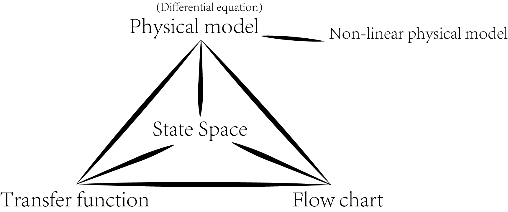
- State Space Model
Usually, a linear system is writen as: $$\dot X = AX + BU$$ $$Y = CX + DU$$ where the matrix A is called as the System Matrix,the matrix B is called as the Input matrix,the matrix C is called as the Output matrix,the matrix D is called as the Feedthrough matrix,the vector X is called as the State variable,the vector U is called as the Input,the vector Y is called as the Output。
- Physical equation description
The state space model resembles an ordinary differential equation. In linear space, we can upsize the state variable X into a vector, such as:$X=[X,\dot X, \ddot X]^T$,Then this equation of state can be written as :$$\left ( \begin{matrix} \dot X \\ \ddot X \\ \dddot X \end{matrix} \right ) = \left [\begin{matrix} 0&1&0\\ 0&0&1\\ a_0&a_1&a_2 \end{matrix}\right] \left(\begin{matrix} X \\ \dot X \\ \ddot X \end{matrix} \right ) + \left [\begin{matrix} 0 \\ 0 \\ 1\end{matrix}\right]U$$. So, it is easy to find out that his physical model is:$$\dddot X = a_0X + a_1\dot X + a_2\ddot X + U$$
In real life, there are many examples where the physical equation is constructed by a high-order ordinary differential equation. For the description of this type of physical phenomenon, we abstract a mathematical model: $$y^{(n)} +a_1y^{(n-1)} + \cdots +a_ny^{(0)}=b_0u^{(n)} +b_1u^{(n-1)} +\cdots +b_nu^{(0)}$$ if $$\begin{cases} \beta_0=b_0 \\ \beta_1=b_1-a_1\beta_0 \\ \beta_2 = b_2-a_2\beta_0-a_1\beta_1 \\ \vdots \end{cases}且 \begin{cases} x_1 =y -\beta_0u \\ x_2 = \dot y -\beta_1u - \beta_0\dot u \\ x_3 = \ddot y -\beta_2u -\beta_1 \dot u -\beta_0 \ddot u \\ \vdots \\ x_n = y^{(n-1)} -\beta_{n-1}u -\beta_{n-2} \dot u - \cdots -\beta_0u^{(n-1)}\end{cases}$$ thus:$$\begin{cases} \dot X=\begin{bmatrix} 0&1&0&\cdots&0 \\ 0&0&1&\cdots&0 \\ \vdots&\vdots&\vdots&\ddots&\vdots \\ -a_n&-a_{n-1}&-a_{n-2}&\cdots&-a_1\end{bmatrix}X+\begin{bmatrix} \beta_1\\ \beta_2\\ \beta_3\\ \vdots\\ \beta_n \end{bmatrix}U \\ Y=\begin{bmatrix}1&0&0&\cdots&0\end{bmatrix}X+\beta_0U \end{cases}$$ If the ** input variable does not contain a high-order derivative term**, then mathematical model is writen as:$$y^{(n)} +a_1y^{(n-1)} + \cdots +a_ny^{(0)}=bu$$ State space model is writen as:$$\begin{pmatrix} \dot y \\ \ddot y \\ \vdots \\ y^{(n)}\end{pmatrix} = \begin{bmatrix} 0&1&0&\cdots&0 \\ 0&0&1&\cdots&0 \\ \vdots&\vdots&\vdots&\ddots&\vdots \\ -a_n&-a_{n-1}&-a_{n-2}&\cdots&-a_1 \end{bmatrix} \begin{pmatrix} y \\ \dot y\\ \vdots \\ y^{(n-1)}\end{pmatrix}+ \begin{bmatrix} 0 \\ 0 \\ \vdots \\ b\end{bmatrix}u$$
** Obviously, physical equations without input derivative terms are easier to use to build state space models**
Example
For higher order differential equations:$\dddot y + 3\ddot y + 5\dot y + 7y = 2\dot u + 4u$,exists:$$\begin{cases}A=\begin{bmatrix} 0&1&0\\0&0&1\\-7&-5&-3\end{bmatrix} B=\begin{bmatrix} 0\\2\\-2\end{bmatrix}\\C=\begin{bmatrix}1&0&0\end{bmatrix} \end{cases}$$
A=[0 1 0;    0 0 1;    -7 -5 -3];
B=[0;2;-2];
C=[1 0 0];
sys=ss(A,B,C,[]);% state space model
tf(sys) % transfer function
ans =

         2 s + 4
  ---------------------
  s^3 + 3 s^2 + 5 s + 7

Continuous-time transfer function.
- Input and output transfer function model
In the linear space, we take the Laplace transform on the input and output of the physical equation to obtain the input-output transfer function in the frequency domain.:$$G(s)=\frac{Y(s)}{U(s)}=\frac{b_0s^n+b_1s^{n-1}+\cdots+b_ns}{a_0s^n+a_1s^{n-1}+\cdots+a_ns}=G_{\Sigma(A,B,C)}(s)+\frac{b_0}{a_0}$$
So we call the equation $a_0s^n+a_1s^{n-1}+\cdots+a_ns=0$ as the characteristic equation of the system,and the roots of the equation are called the feature value or Pole. Accordingly, the roots of the equation $b_0s^n+b_1s^{n-1}+\cdots+b_ns=0$ is called Zero point.
When the denominator is written as $s^2+a_1s+a_2$,it exists $\omega=\sqrt{a_2},\xi=\frac{a_1}{2\omega}$. $\omega$ is called as natural frequency,$\xi$ is called as damping ratio. when $\xi=1$ represents the critical damping, but when $\xi>1$, the system has a large damping ratio。

- In the transfer function $G_{\Sigma(A,B,C)}(s)$,if poles are different (root does not repeat), transfer function can be written as:
if:$\begin{cases} X_i(s)=\frac{1}{s-s_i}U(s) \Rightarrow \dot x_i=s_ix_i + u \\ Y(s)=\sum k_iX_i(s)+Du \Rightarrow y=k_1x_1+k_2x_2+\cdots+k_nx_n+Du\end{cases}$
$$\Rightarrow \begin{cases}\dot X=\begin{bmatrix}s_1&&&\\&s_2&&\\&&\ddots&\\&&&s_n\end{bmatrix}X+\begin{bmatrix}1\\1\\ \vdots\\1\end{bmatrix}u \\ Y=\begin{bmatrix}k_1&k_2&\cdots&k_n\end{bmatrix}X+Du\end{cases}$$
- if it exists ** same poles**,i.e:$G(s)=\frac{k_{11}}{(s-s_1)^3}+\frac{k_{12}}{(s-s_1)^3}+\frac{k_{13}}{(s-s_1)^3}+\frac{k_{41}}{(s-s_4)^3}+\frac{k_{51}}{(s-s_5)^3}+\frac{k_{52}}{(s-s_5)^3}$,$s_1$ 3 tiems,and $s_5$ 2 times。
if:$X_1(s)=\frac{U(s)}{(s-s_1)^3}=\frac{X_2(s)}{s-s_1}\Rightarrow\dot X_1=s_1X_1+S_2$ $$\Rightarrow \begin{cases}\dot X=\begin{bmatrix} s_1&1\\&s_1&1\\&&s_1\\&&&s_4\\&&&&s_5&1\\&&&&&s_5\end{bmatrix}X+\begin{bmatrix}0\\0\\1\\1\\0\\1\end{bmatrix}u \\ Y=\begin{bmatrix}k_{11}&k_{12}&\cdots&k_{52}\end{bmatrix}X\end{cases}$$
- If there is a zero-pole pair (zero pole coincidence), the corresponding pole-zero pair is Eliminated.
Matlab code
sys_min=minreal(sys)
Obviously, we can see that for a physical equation with derivative input terms, it is easier to get a state space model by constructing an input-output transfer function.
However, the input-output transfer function model can only establish a single-input single-output system (SISO), so usually for multiple-input multiple-output systems (MIMO), we need to build a transfer function model for each combination of input and output.
Example
Still for this higher order differential equation$\dddot y + 3\ddot y + 5\dot y + 7y = 2\dot u + 4u$. After the Laplace transform: $$G(s)=\frac{Y(s)}{U(s)}=\frac{2s+4}{s^3+3s^2+5s+7}$$ Matlab code
num=[2 4];den=[1 3 5 7];
num=[2 4];den=[1 3 5 7];
system_1=tf(num,den)
system_1 =

         2 s + 4
  ---------------------
  s^3 + 3 s^2 + 5 s + 7

Continuous-time transfer function.
State space model is transformed into transfer function model
State space model :$$\begin{cases}\dot X = AX + BU \\Y = CX + DU \end{cases}\Rightarrow \begin{cases}sX = AX + BU \\Y = CX + DU \end{cases}$$
transfer function model:$$G(s)=\frac{Y(s)}{U(s)}=C(sI-A)^{-1}B+D$$
system_2=tf(sys)
system_2 =

         2 s + 4
  ---------------------
  s^3 + 3 s^2 + 5 s + 7

Continuous-time transfer function.
- Flow chart model
Take dual input and dual output as an example:
$\begin{cases}\ddot y_1 +a_1\dot y_1 +a_2y_2 =b_1\dot u_1 +b_2u_1 +b_3u_2 \\ \dot y_2 +a_3y_2 +a_4y_1 =b_4u_2\end{cases}$
$\Rightarrow$
$\begin{cases}y_1=\lmoustache(-a_1y_1+b_1u_1)dt +\lmoustache\lmoustache(b_2u_1+b_3u_2-a_2y_2)dt^2 \\ y_2=\lmoustache(-a_3y_2-a_4y_1+b_4u_2)dt\end{cases}$
Think of each integration result as a state variable, then:
$\begin{cases}\dot x_1=-a_1x_1+x_2+b_1u_1 \\ \dot x_2=-a_2x_3+u_1b_2+u_2b_3 \\ \dot x_3=-a_4x_1-a_3x_3+u_2b_4 \\ y_1=x_1\\y_2=x_3\end{cases}$
$\Rightarrow$
$\begin{cases}\dot X=\begin{bmatrix}-a_1&1&0\\0&0&-a_2\\-a_4&0&-a_3\end{bmatrix}X +\begin{bmatrix}b_1&0\\b_2&b_3\\0&b_4\end{bmatrix} \begin{pmatrix}u_1\\u_2\end{pmatrix} \\ Y=\begin{bmatrix}1&0&0\\0&0&1\end{bmatrix}X\end{cases}$
Obviously, for MIMO systems, the flow chart model makes it easier to construct a state space model than the input-output transfer function model.
Linear system combination model
- Parallel:$G(s)=G_1(s)+G_2(s)$
parallel(sys1,sys2)
- serise:$G(s)=G_1(s)G_2(s)$
series(sys1,sys2)
- feedback:$G(s)=(I+G_1(s)G_2(s))^{-1}G_1(s)$
feedback(sys1,sys2)
- Nonlinear system model
Nonlinear systems are a more general system than linear systems. Usually a nonlinear system cannot directly write its state space model. It first needs to be linearized so that we can write an approximate state space model near a certain equilibrium point.
Take the kinetic equation as an example:
$$A(q)\ddot q+C(q,\dot q)\dot q+g(q)=Qu$$
state variable $x=[q,\dot q]^T$, it exists the stable input $u_e$ at the equilibrim point $x_e=[q_e,0]^T$
so:
$$\dot X=F(x)+G(x)u=\begin{bmatrix} \dot q \\ A(q)^{-1}(-C(q,\dot q)\dot q-g(q))\end{bmatrix} +\begin{bmatrix} 0 \\ A(q)^{-1}Q\end{bmatrix}u$$
Example (Inverted pendulum)
$$\begin{cases} (J+ml^2)\frac{d^2\theta}{dt^2}+(mlcos\theta)\frac{d^2x}{dt^2}=mldsin\theta \\ (M+m)\frac{d^2x}{dt^2}+\mu_c\frac{dx}{dt}+(mlcos\theta)\frac{d^2\theta}{dt^2}=u+mlsin\theta(\frac{d\theta}{dt})^2\end{cases}$$Linear Transformation of State Space Model and Jordan Canonical form
In order to reduce the difficulty of system analysis and design, the general form of the state space model is transformed into a specific form of the model, and does not change the characteristics of the system itself (transmission characteristics), this process is called the linear transformation of the state space model. The Jordan canonical form is one of the specific forms of the model.
- Linear transformation
Original state space model:$$\sum(A,B,C,D):\begin{cases}\dot X = AX + BU \\Y = CX + DU \end{cases}$$
after Linear transformation:$\bar{X}=PX$
obtain:$$\sum(\bar{A},\bar{B},\bar{C},\bar{D}):\begin{cases} \dot {\bar{X}} = \bar{A} \bar{X} + \bar{B} U \\ Y = \bar{C} \bar{X} + \bar{D} U \end{cases}$$
where:
$$\bar{A}=PAP^{-1},\bar{B}=PB,\bar{C}=CP^{-1},bar{D}=D$$
so:$$\bar{G}=\frac{Y}{U}=\bar{C}(sI-\bar{A})^{-1}\bar{B}+\bar{D}=C(sI-A)^{-1}B+D=G$$
Matlab code:
sys_new=ss2ss(sys_old,P)
- Diagonal Canonical form
The system matrix A is transformed into a diagonal matrix, which means that $\bar{A}$ is the eigenvalue matrix of the matrix A. Therefore, the matlab function is used:
[P,D]=eig(A)
obtain the diagonal matrix $D=\bar{A}=PAP^{-1}$
- Jordan Canonical form
[P,J]=jordan(A)
obtain the Jordan matrix $J=\bar{A}=PAP^{-1}$
A = [1 -3 -2; -1 1 -1; 2 4 5]
[P,J]=jordan(A)
A =

     1    -3    -2
    -1     1    -1
     2     4     5


P =

    -1     1    -1
    -1     0     0
     2     0     1


J =

     2     1     0
     0     2     0
     0     0     3