Методы машинного обучения
Семинар: деревья решений
%matplotlib inline
import pandas as pd
import numpy as np
import matplotlib.pyplot as plt

plt.style.use('ggplot')
plt.rcParams['figure.figsize'] = (12,8)
Titanic Dataset
from sklearn.tree import DecisionTreeClassifier
from sklearn.tree import export_graphviz
import subprocess
- Load titanic dataset
df = pd.read_csv('./data/titanic.csv')
df.head()
| PassengerId | Survived | Pclass | Name | Sex | Age | SibSp | Parch | Ticket | Fare | Cabin | Embarked | |
|---|---|---|---|---|---|---|---|---|---|---|---|---|
| 0 | 1 | 0 | 3 | Braund, Mr. Owen Harris | male | 22.0 | 1 | 0 | A/5 21171 | 7.2500 | NaN | S |
| 1 | 2 | 1 | 1 | Cumings, Mrs. John Bradley (Florence Briggs Th... | female | 38.0 | 1 | 0 | PC 17599 | 71.2833 | C85 | C |
| 2 | 3 | 1 | 3 | Heikkinen, Miss. Laina | female | 26.0 | 0 | 0 | STON/O2. 3101282 | 7.9250 | NaN | S |
| 3 | 4 | 1 | 1 | Futrelle, Mrs. Jacques Heath (Lily May Peel) | female | 35.0 | 1 | 0 | 113803 | 53.1000 | C123 | S |
| 4 | 5 | 0 | 3 | Allen, Mr. William Henry | male | 35.0 | 0 | 0 | 373450 | 8.0500 | NaN | S |
- Проанализируем данные
- Типы признаков
- Пропущенные значения?
- Пропорции классов
df.isnull().mean()
PassengerId    0.000000
Survived       0.000000
Pclass         0.000000
Name           0.000000
Sex            0.000000
Age            0.198653
SibSp          0.000000
Parch          0.000000
Ticket         0.000000
Fare           0.000000
Cabin          0.771044
Embarked       0.002245
dtype: float64
df.Survived.value_counts()
0    549
1    342
Name: Survived, dtype: int64
- Предобработка данных
- выкидываем ненужные признаки
- готовимся к работе с пропусками
- подготовка категориальных признаков
- разбиваем на обучение и контроль
df.Embarked.mode()
0    S
dtype: object
drop_cols = ['PassengerId', 'Name', 'Ticket', 'Cabin']

df.loc[:, 'Age'] = df.Age.fillna(df.Age.mean())
df.loc[:, 'Embarked'] = df.Embarked.fillna(df.Embarked.mode()[0])
df = pd.get_dummies(df, columns=['Embarked'])

df.loc[:, 'Sex'] = df.Sex.replace({'male': 1, 'female': 0})

df_result = df.drop(drop_cols, axis=1)
df_result.head()
| Survived | Pclass | Sex | Age | SibSp | Parch | Fare | Embarked_C | Embarked_Q | Embarked_S | |
|---|---|---|---|---|---|---|---|---|---|---|
| 0 | 0 | 3 | 1 | 22.0 | 1 | 0 | 7.2500 | 0 | 0 | 1 |
| 1 | 1 | 1 | 0 | 38.0 | 1 | 0 | 71.2833 | 1 | 0 | 0 |
| 2 | 1 | 3 | 0 | 26.0 | 0 | 0 | 7.9250 | 0 | 0 | 1 |
| 3 | 1 | 1 | 0 | 35.0 | 1 | 0 | 53.1000 | 0 | 0 | 1 |
| 4 | 0 | 3 | 1 | 35.0 | 0 | 0 | 8.0500 | 0 | 0 | 1 |
X = df_result.iloc[:, 1:].values
y = df_result.iloc[:, 0].values
from sklearn.model_selection import train_test_split
X_train, X_valid, y_train, y_valid = train_test_split(X, y, test_size=0.2, random_state=123)
- Обучим модель и визуализируем ее
- Посмотрим на важность признаков
def plot_tree(tree, feature_names=None, class_names=['0', '1']):
    with open('tree.dot', 'w') as fout:
        export_graphviz(tree, out_file=fout, filled=True, feature_names=feature_names, class_names=class_names)
    command = ["dot", "-Tpng", "tree.dot", "-o", "tree.png"]
    subprocess.check_call(command)
    plt.imshow(plt.imread('tree.png'))
    plt.axis("off")
from sklearn.tree import DecisionTreeClassifier
model = DecisionTreeClassifier(max_depth=4)
model.fit(X_train, y_train)
DecisionTreeClassifier(class_weight=None, criterion='gini', max_depth=4,
            max_features=None, max_leaf_nodes=None,
            min_impurity_decrease=0.0, min_impurity_split=None,
            min_samples_leaf=1, min_samples_split=2,
            min_weight_fraction_leaf=0.0, presort=False, random_state=None,
            splitter='best')
y_hat = model.predict_proba(X_valid)
y_hat[:10]
array([[0.38541667, 0.61458333],
       [0.86486486, 0.13513514],
       [0.60465116, 0.39534884],
       [0.60465116, 0.39534884],
       [0.86486486, 0.13513514],
       [0.93902439, 0.06097561],
       [0.11111111, 0.88888889],
       [0.11111111, 0.88888889],
       [0.38541667, 0.61458333],
       [0.38541667, 0.61458333]])
from sklearn.metrics import roc_auc_score, roc_curve
fpr, tpr, thresh = roc_curve(y_valid, y_hat[:, 1])
plt.plot(fpr, tpr)
plt.xlabel('FPR')
plt.ylabel('TPR')
Text(0,0.5,'TPR')

roc_auc_score(y_valid, y_hat[:, 1])
0.8749662618083671
pd.Series(index=df_result.columns[1:], data=model.feature_importances_)
Pclass        0.195365
Sex           0.577291
Age           0.095079
SibSp         0.072319
Parch         0.005876
Fare          0.054071
Embarked_C    0.000000
Embarked_Q    0.000000
Embarked_S    0.000000
dtype: float64
plot_tree(model, feature_names=df_result.columns[1:])

Speed Dating Data
Предобработка данных
df = pd.read_csv('./data/speed-dating-experiment/Speed Dating Data.csv', encoding='latin1')
df.shape
(8378, 195)
df = df.iloc[:, :97]
Рассмотрим нужные признаки по очереди
df.iid.nunique()
551
df = df.drop(['id'], axis=1)
df = df.drop(['idg'], axis=1)
gender
- Female=0
- Male=1
df.drop_duplicates(subset=['iid']).gender.value_counts()
1    277
0    274
Name: gender, dtype: int64
df.drop_duplicates(subset=['iid']).condtn.value_counts()
2    386
1    165
Name: condtn, dtype: int64
df = df.drop(['condtn'], axis=1)
wave
Пока оставим в таблице, но в качестве признака рассматривать не будем
df.wave.unique()
array([ 1,  2,  3,  4,  5,  6,  7,  8,  9, 10, 11, 12, 13, 14, 15, 16, 17,
       18, 19, 20, 21])
df = df.drop(['round'], axis=1)
df = df.drop(['position', 'positin1'], axis=1)
order:
the number of date that night when met partner
df = df.drop(['order'], axis=1)
df = df.drop(['partner'], axis=1)
df = df.drop(['age_o', 'race_o', 'pf_o_att',
              'pf_o_sin', 'pf_o_int',
              'pf_o_fun', 'pf_o_amb', 'pf_o_sha',
              'dec_o', 'attr_o', 'sinc_o', 'intel_o', 'fun_o',
              'amb_o', 'shar_o', 'like_o', 'prob_o','met_o'],
             axis=1)
age
оставляем
df.drop_duplicates(subset=['iid']).age.hist(bins=20)
<matplotlib.axes._subplots.AxesSubplot at 0x1a1b1a4e80>

df.drop_duplicates('iid').age.isnull().sum()
8
df = df.dropna(subset=['age'])
for i, group in df.groupby('field_cd'):
    print('=' * 10)
    print('Field Code {}'.format(i))
    print(group.field.unique())
==========
Field Code 1.0
['Law' 'law' 'LAW' 'Law and Social Work'
 'Law and English Literature (J.D./Ph.D.)' 'Intellectual Property Law'
 'Law/Business']
==========
Field Code 2.0
['Economics' 'Mathematics' 'Statistics' 'math' 'Mathematics, PhD' 'Stats'
 'math of finance' 'Math']
==========
Field Code 3.0
['Psychology' 'Speech Language Pathology' 'Speech Languahe Pathology'
 'Educational Psychology' 'Organizational Psychology' 'psychology'
 'Communications' 'Sociology' 'psychology and english' 'theory'
 'Health policy' 'Clinical Psychology' 'Sociology and Education'
 'sociology' 'Anthropology/Education' 'speech pathology'
 'Speech Pathology' 'Anthropology' 'School Psychology' 'anthropology'
 'Counseling Psychology' 'African-American Studies/History']
==========
Field Code 4.0
['Medicine' 'Art History/medicine'
 'Sociomedical Sciences- School of Public Health' 'Epidemiology'
 'GS Postbacc PreMed' 'medicine']
==========
Field Code 5.0
['Operations Research' 'Mechanical Engineering' 'Engineering'
 'Electrical Engineering' 'Operations Research (SEAS)'
 'Education Administration' 'Computer Science' 'Biomedical Engineering'
 'electrical engineering' 'engineering' 'Medical Informatics'
 'medical informatics' 'Electrical Engg.' 'Environmental Engineering'
 'Instructional Tech & Media' 'MA in Quantitative Methods'
 'Urban Planning' 'Financial Engineering' 'biomedical engineering'
 'biomedical informatics' 'ELECTRICAL ENGINEERING'
 'Biomedical engineering' 'Industrial Engineering'
 'Industrial Engineering/Operations Research'
 'Masters of Industrial Engineering' 'Biomedical Informatics']
==========
Field Code 6.0
['MFA Creative Writing' 'Classics' 'Journalism' 'English'
 'Comparative Literature' 'English and Comp Lit'
 'Communications in Education' 'Creative Writing'
 'Creative Writing - Nonfiction' 'Writing: Literary Nonfiction'
 'Creative Writing (Nonfiction)' 'NonFiction Writing' 'SOA -- writing'
 'journalism' 'Nonfiction writing']
==========
Field Code 7.0
['German Literature' 'Religion' 'philosophy' 'History of Religion'
 'Modern Chinese Literature' 'Philosophy' 'Religion, GSAS' 'History'
 'History (GSAS - PhD)' 'American Studies' 'Philosophy (Ph.D.)'
 'Philosophy and Physics' 'Art History' 'art history']
==========
Field Code 8.0
['Finance' 'Business' 'money' 'Applied Maths/Econs' 'Economics' 'Finanace'
 'Finance&Economics' 'Mathematical Finance' 'MBA'
 'Business & International Affairs' 'Marketing' 'Business (MBA)'
 'financial math' 'Business- MBA' 'Economics, English'
 'Economics, Sociology' 'Economics and Political Science' 'business'
 'Business, marketing' 'Business/ Finance/ Real Estate'
 'International Affairs/Finance' 'international finance and business'
 'International Business' 'International Finance, Economic Policy'
 'Business/Law' 'Business and International Affairs (MBA/MIA Dual Degree)'
 'QMSS' 'Public Administration' 'Master in Public Administration'
 'Business School' 'MBA / Master of International Affairs (SIPA)'
 'Finance/Economics' 'Business Administration' 'MBA Finance'
 'BUSINESS CONSULTING' 'business school' 'Business, Media'
 'Fundraising Management' 'Business (Finance & Marketing)' 'Consulting'
 'MBA - Private Equity / Real Estate' 'General management/finance']
==========
Field Code 9.0
['TC (Health Ed)' 'Elementary/Childhood Education (MA)'
 'International Educational Development' 'Art Education'
 'elementary education' 'MA Science Education' 'Social Studies Education'
 'MA Teaching Social Studies' 'Education Policy'
 'Education- Literacy Specialist' 'bilingual education' 'Education'
 'math education' 'TESOL' 'Elementary Education'
 'Cognitive Studies in Education' 'education'
 'Curriculum and Teaching/Giftedness' 'Instructional Media and Technology'
 'English Education' 'art education' 'Early Childhood Education'
 'Ed.D. in higher education policy at TC' 'EDUCATION' 'music education'
 'Music Education' 'Higher Ed. - M.A.' 'Neuroscience and Education'
 'Elementary Education - Preservice'
 'Education Leadership - Public School Administration'
 'Bilingual Education' 'teaching of English']
==========
Field Code 10.0
['chemistry' 'microbiology' 'Chemistry'
 'Climate-Earth and Environ. Science' 'marine geophysics'
 'Nutrition/Genetics' 'Neuroscience' 'physics (astrophysics)' 'Physics'
 'Biochemistry' 'biology' 'Cell Biology' 'Microbiology' 'climate change'
 'MA Biotechnology' 'Ecology' 'Computational Biochemsistry' 'Neurobiology'
 'biomedicine' 'Biology' 'Conservation biology' 'biotechnology'
 'Earth and Environmental Science' 'nutrition' 'Genetics' 'Nutritiron'
 'Molecular Biology' 'Genetics & Development' 'genetics'
 'medicine and biochemistry' 'Epidemiology' 'Nutrition'
 'Applied Physiology & Nutrition' 'Biomedical Engineering' 'physics'
 'Biotechnology' 'Neurosciences/Stem cells' 'Biology PhD'
 'biochemistry/genetics' 'epidemiology'
 'Biochemistry & Molecular Biophysics']
==========
Field Code 11.0
['social work' 'Social Work' 'Masters of Social Work' 'Social work'
 'International Affairs' 'Social Work/SIPA']
==========
Field Code 12.0
['Undergrad - GS']
==========
Field Code 13.0
['Masters in Public Administration' 'Masters of Social Work&Education'
 'political science' 'International Relations'
 'international affairs - economic development' 'Political Science'
 'American Studies (Masters)' 'International Affairs'
 'international affairs/international finance' 'International Development'
 'International Affairs and Public Health' 'International affairs'
 'International Affairs/Business' 'Master of International Affairs'
 'International Politics' 'SIPA / MIA'
 'International Security Policy - SIPA' 'Intrernational Affairs'
 'International Affairs - Economic Policy' 'SIPA - Energy' 'Public Policy'
 'Human Rights: Middle East' 'Human Rights' 'SIPA-International Affairs'
 'Public Administration']
==========
Field Code 14.0
['Film' 'MFA -Film' 'film']
==========
Field Code 15.0
['Arts Administration' 'Museum Anthropology'
 'Theatre Management & Producing' 'MFA Writing' 'MFA  Poetry' 'Theater'
 'MFA Acting Program' 'Acting' 'Public Health']
==========
Field Code 16.0
['Polish' 'Japanese Literature' 'french']
==========
Field Code 17.0
['Architecture']
==========
Field Code 18.0
['working' 'GSAS' 'Climate Dynamics']
df.field_cd.isnull().sum()
19
df.loc[:, 'field_cd'] = df.loc[:, 'field_cd'].fillna(19)
df = df.drop(['field'], axis=1)
Надо же как-то закодировать field_cd!
from sklearn.preprocessing import OneHotEncoder
df = \
pd.get_dummies(df, prefix='field_code', prefix_sep='=',
               columns=['field_cd'])
df.head()
| iid | gender | wave | pid | match | int_corr | samerace | age | undergra | mn_sat | ... | field_code=10.0 | field_code=11.0 | field_code=12.0 | field_code=13.0 | field_code=14.0 | field_code=15.0 | field_code=16.0 | field_code=17.0 | field_code=18.0 | field_code=19.0 | |
|---|---|---|---|---|---|---|---|---|---|---|---|---|---|---|---|---|---|---|---|---|---|
| 0 | 1 | 0 | 1 | 11.0 | 0 | 0.14 | 0 | 21.0 | NaN | NaN | ... | 0 | 0 | 0 | 0 | 0 | 0 | 0 | 0 | 0 | 0 |
| 1 | 1 | 0 | 1 | 12.0 | 0 | 0.54 | 0 | 21.0 | NaN | NaN | ... | 0 | 0 | 0 | 0 | 0 | 0 | 0 | 0 | 0 | 0 |
| 2 | 1 | 0 | 1 | 13.0 | 1 | 0.16 | 1 | 21.0 | NaN | NaN | ... | 0 | 0 | 0 | 0 | 0 | 0 | 0 | 0 | 0 | 0 |
| 3 | 1 | 0 | 1 | 14.0 | 1 | 0.61 | 0 | 21.0 | NaN | NaN | ... | 0 | 0 | 0 | 0 | 0 | 0 | 0 | 0 | 0 | 0 |
| 4 | 1 | 0 | 1 | 15.0 | 1 | 0.21 | 0 | 21.0 | NaN | NaN | ... | 0 | 0 | 0 | 0 | 0 | 0 | 0 | 0 | 0 | 0 |
5 rows × 88 columns
df.undergra.value_counts().head()
UC Berkeley    107
Harvard        104
Columbia        95
Yale            86
NYU             78
Name: undergra, dtype: int64
df = df.drop(['undergra'], axis=1)
mn_sat:
Median SAT score for the undergraduate institution where attended.
df.mn_sat.value_counts().head()
1,400.00    403
1,430.00    262
1,290.00    190
1,450.00    163
1,340.00    146
Name: mn_sat, dtype: int64
df.loc[:, 'mn_sat'] = df.loc[:, 'mn_sat'].str.replace(',', '').astype(np.float)
df.drop_duplicates('iid').mn_sat.hist()
<matplotlib.axes._subplots.AxesSubplot at 0x1a1b1ff860>

df.drop_duplicates('iid').mn_sat.isnull().sum()
342
# Что будем делать?
df = df.drop(['mn_sat'], axis=1)
tuition:
Tuition listed for each response to undergrad in Barron’s 25th Edition college profile book.
df.tuition.value_counts().head()
26,908.00    241
26,019.00    174
15,162.00    138
25,380.00    112
26,062.00    108
Name: tuition, dtype: int64
df.loc[:, 'tuition'] = df.loc[:, 'tuition'].str.replace(',', '').astype(np.float)
df.drop_duplicates('iid').tuition.hist()
<matplotlib.axes._subplots.AxesSubplot at 0x103a6bcc0>

df.drop_duplicates('iid').tuition.isnull().sum()
310
# Что будем делать?
df = df.drop(['tuition'], axis=1)
race:
- Black/African American=1
- European/Caucasian-American=2
- Latino/Hispanic American=3
- Asian/Pacific Islander/Asian-American=4
- Native American=5
- Other=6
# Ну тут вы уже сами знаете как быть
df = pd.get_dummies(df, prefix='race', prefix_sep='=',
                    columns=['race'])
df.drop_duplicates('iid').imprace.isnull().sum()
1
df.drop_duplicates('iid').imprelig.isnull().sum()
1
# Что делать?

df = df.dropna(subset=['imprelig', 'imprace'])
df = df.drop(['from', 'zipcode'], axis=1)
income
df.loc[:, 'income'] = df.loc[:, 'income'].str.replace(',', '').astype(np.float)
df.drop_duplicates('iid').loc[:, 'income'].hist()
<matplotlib.axes._subplots.AxesSubplot at 0x1a1b28e128>

df.drop_duplicates('iid').loc[:, 'income'].isnull().sum()
261
df = df.drop(['income'], axis=1)
# df.loc[:, 'income'] = df.loc[:, 'income'].fillna(-999)
goal:
What is your primary goal in participating in this event?
Seemed like a fun night out=1
To meet new people=2
To get a date=3
Looking for a serious relationship=4
To say I did it=5
Other=6
date:
In general, how frequently do you go on dates?
Several times a week=1
Twice a week=2
Once a week=3
Twice a month=4
Once a month=5
Several times a year=6
Almost never=7
go out:
How often do you go out (not necessarily on dates)?
Several times a week=1
Twice a week=2
Once a week=3
Twice a month=4
Once a month=5
Several times a year=6
Almost never=7
Как бы вы предложили закодировать эти переменные?
df.drop_duplicates('iid').goal.isnull().sum()
0
df = pd.get_dummies(df, prefix='goal',
                    prefix_sep='=', columns=['goal'])
df = df.dropna(subset=['date'])
df.drop_duplicates('iid').go_out.isnull().sum()
0
for i, group in df.groupby('career_c'):
    print('=' * 10)
    print('Career Code {}'.format(i))
    print(group.career.unique())
==========
Career Code 1.0
['lawyer/policy work' 'lawyer' 'Law' 'Corporate Lawyer' 'Lawyer'
 'Corporate attorney' 'law' 'Intellectual Property Attorney' 'LAWYER'
 'attorney' 'Lawyer or professional surfer' 'lawyer/gov.position'
 'Law or finance' 'IP Law' 'Academic (Law)' 'Private Equity' 'attorney?'
 'Corporate law' 'tax lawyer' 'Business/Law' 'Assistant District Attorney']
==========
Career Code 2.0
['Academia, Research, Banking, Life' 'academics or journalism' 'Professor'
 'Academic' 'academia' 'teacher' 'industrial scientist'
 'teaching and then...' 'Professor of Media Studies'
 'Education Administration' 'Academic or Research staff'
 'University Professor' 'Research Scientist'
 'research in industry or academia' 'Teacher/Professor'
 'no idea, maybe a professor' 'a research position' 'professor' 'teaching'
 'engineering professional' 'research' 'Neuroscientist/Professor'
 'Education' 'Professor and Government Official'
 'physicist, probably academia' 'college art teacher' 'academic'
 'Research scientist, professor' 'academics' 'academic research'
 'academician' 'professional student' 'education' 'Historian'
 'college professor' 'scientific research' 'Academic Physician'
 'Researcher' 'Professor or Consultant' 'History Professor'
 'Educational Policy' 'elementary school teacher' 'Research/Teaching'
 'researcher in sociology' 'scientist' 'Naturalist'
 'professor, poet/critic' 'researcher/academia' 'Art educator and Artist'
 'Teacher' 'Scientist' 'Scientist/educator'
 'scientific research for now but who knows' 'College Professor'
 'Professor or Lawyer' 'research position in pharmaceutical industry'
 'Academia' 'research/academia' 'Secondary Education Teacher'
 'High School Social Studies Teacher' 'Education Policy Analyst'
 'Literacy Organization head/ Director of Development for non-profit'
 'English Teacher' 'Program development / policy work'
 'professor of education' 'Educator' 'teaching/education'
 'professor in college' 'Academia; Research; Teaching'
 'curriculum developer' 'academic or consulting' 'Academia or UN'
 'I am a teacher.' 'Professor or journalist'
 'to get Ph.D and be a professor'
 'Early Childhood Ed. - College/univ. faculity'
 'medical examiner or researcher' 'University President'
 'EDUCATION ADMINISTRATION' 'music educator, performer'
 'Elementary Education Teaching' 'research - teaching' 'Research'
 'Elementary school teacher' 'Bilingual Elementary School Teacher'
 'Professor, or Engineer' 'Professor; Human Rights Director'
 'Clinic Trial' 'English teacher' 'writer/teacher' 'Professor...?'
 'acadeic' 'researcher' 'biology industry' 'Epidemiologist'
 'epidemiologist' 'teacher and performer' 'TEACHING' 'Academic/ Finance'
 'Science' 'Academic Work, Consultant']
==========
Career Code 3.0
['psychologist' 'Social Worker.... Clinician' 'Psychologist'
 'school psychologist' 'School Psychologist' 'Clinical Psychology'
 'Clinical Psychologist' 'clinical psychologist, researcher, professor'
 'School Counseling' 'Sex Therapist']
==========
Career Code 4.0
['Biostatistics' 'Medicine' 'pharmaceuticals' 'Cardiologist' 'Pediatrics'
 'medicine' 'pharmaceuticals and biotechnology' 'Physician Scientist'
 'health policy' 'Epidemiologist' 'nutrition and dental' 'Physician'
 'dietician' 'doctor and entrepreneur' 'Healthcare' 'Nutritionist'
 'Private practice Dietician' 'physician, informaticist' 'physician'
 'Medical Sciences' 'physician/healthcare' 'Doctor']
==========
Career Code 5.0
['Informatics' 'Engineer' 'Ph.D. Electrical Engineering'
 'Operations Research' 'Engineering' 'Mechanical Engineering'
 'Civil Engineer' 'Urban Planner' 'Planning' 'ASIC Engineer'
 'software engr, network engr' 'Research Engineer']
==========
Career Code 6.0
['Journalist' "Clidren's TV" 'Music production' 'comedienne' 'novelist'
 'Journalism' 'film' 'Writer' 'Porn Star' 'boxing champ'
 'Paper Back Writer'
 'Poet, Writer, Singer, Policy Maker with the UN and/or Indian Govt.'
 'Entertainment/Sports' 'WRITING' 'manage a museum or art gallery'
 'Entertainment/Media' 'Film/Television' 'Writing'
 'Museum Work (Curation?)' 'Music Industry' 'Artist' 'Art Management'
 'film directing' 'Screenwriter' 'Filmmaker' 'Writer/teacher'
 'Writing or Editorial' 'writer/editor'
 'producer at a non-profit regional theatre' 'writer' 'playing music'
 'writer/producer' 'film and radio' 'Film' 'Writer/Editor' 'Actress'
 'Acting']
==========
Career Code 7.0
['research/financial industry' 'Financial Services' 'ceo' 'CEO' 'Banking'
 'Capital Markets' 'Organizational Change Consultant' 'banker / academia'
 'banker' 'Entrepreneur' 'consulting' 'Private Equity Investing'
 'Investment Banking' 'Engineer or iBanker or consultant' 'Trading'
 'Economic research' 'Microfinancing Program Manager' 'Marketing'
 'Business - Investment Management' 'Finance' 'business'
 'Marketing, Advertising' 'Asset Management' 'investment banking' 'MBA'
 'Business' 'finance' 'Marketing and Media' 'Brand Management'
 'Management Consulting' 'management consulting'
 'financial service or fashion' 'International Business' 'Private Equity'
 'Investment Management' 'Development work' 'marketing / brand management'
 'Biotech/business' 'Country Analysis/Research/Credit Analysis'
 'Consulting' 'corporate finance'
 'CEO in For Profit Biomedical Organization' 'banking'
 'Conservation training and education' 'president' 'Management Consultant'
 'Trader' 'Wall Street Economist' 'enterpreneur' 'Industry CTO/CEO'
 'finance or engineering' 'Venture Capital/Consulting/Government'
 "Int'l Business" 'Pharmaceuticals/Consulting' 'Investment banking'
 'International Development banker'
 'Corporate Finance, Asset Management/ Hedge Funds'
 'Real Estate Consulting' 'Director of Training and Development'
 'Marketing or Strategy and Business Development' 'Business Consulting'
 'CONSULTING' 'investment management' 'Finance Related'
 'Media Marketing/Entrepreneurship' 'Director of Admissions'
 'Consultin \\ Management'
 'Financial Mathematics-Investment Bank or Hedge Fund-Derivatives Quant Analyst'
 'Work in an investment bank' 'M&A Advisory' 'millionaire'
 'Fundraising for Non-Profits' 'Money Management' 'General Management'
 'Public School Principal' 'Media Management' 'Public Finance'
 'Business Management' 'private equity' 'Health care finance'
 'Entrepreneurship' 'Fixed Income Sales & Trading'
 'Consulting, later Arts or Non-Profit' 'Finance/Economics'
 'Investment Banker' 'consultant'
 'Business Management and Information Technology' 'self-made millionare'
 'To go into Finance' 'Private Equity - Leveraged Buy-Outs' 'Management'
 'General management/consulting']
==========
Career Code 8.0
['Real Estate' 'Real Estate/ Private Equity']
==========
Career Code 9.0
['Congresswoman, and comedian'
 'To create early childhood intervention programs'
 'health/nutrition oriented social worker' 'Social Worker'
 'Social work with children' 'Speech Language Pathologist'
 'Social Work Administration' 'social worker' 'Social Services/ Policy'
 'Clinical Social Worker' 'international development work' 'Nonprofit'
 'Child Rights' 'Development work on field in the middle of nowhere'
 'International Development' 'UN Civil Servant'
 'Humanitarian Affairs/Human Rights'
 'International affairs related career' 'public service'
 'Security Policy - Homeland Defense'
 'reorganizing society. no, I am not being flip.' 'Intl Development'
 "Diplomat / Int'l civil servant" 'Diplomat/Business'
 'Economic Policy Advisor on Latin America' 'Energy Management' 'Diplomat'
 'Work at the UN' 'Foreign Service'
 'Exec. Director of social service non-profit']
==========
Career Code 10.0
['Undecided' "I don't know" 'What a question!' 'if only i knew'
 "don't know" 'Not Sure' 'undecided' 'TBA' 'Am not sure' 'Who knows' '?'
 'not sure yet :)' 'Make money' 'still wondering' 'Not sure yet' 'unknown'
 'unsure' '??' 'dont know yet']
==========
Career Code 11.0
['Social Worker' 'Counseling Adolescents' 'Social work' 'Social Work'
 'Social Work Policy' 'Clinical Social Worker']
==========
Career Code 12.0
['speech pathologist' 'Speech Pathologist']
==========
Career Code 13.0
['GOVERNOR' 'Political Development in Africa' 'Lobbyist' 'politics'
 'School Leadership/Politics']
==========
Career Code 14.0
['Pro Beach Volleyball']
==========
Career Code 15.0
['Hero' 'Energy' 'Trade Specialist' 'professional career'
 "assistant master of the universe (otherwise it's too much work)"]
==========
Career Code 16.0
['journalism' 'Writer/journalist']
==========
Career Code 17.0
['Architecture and design']
df.career_c.isnull().sum()
59
df.loc[:, 'career_c'] = df.loc[:, 'career_c'].fillna(18)
df = df.drop(['career'], axis=1)
# Теперь это надо закодировать
df = pd.get_dummies(df, prefix='career', prefix_sep='=',
                    columns=['career_c'])
How interested are you in the following activities, on a scale of 1-10?
sports: Playing sports/ athletics
tvsports: Watching sports
excersice: Body building/exercising
dining: Dining out
museums: Museums/galleries
art: Art
hiking:  Hiking/camping
gaming: Gaming
clubbing: Dancing/clubbing
reading: Reading
tv: Watching TV
theater: Theater
movies: Movies
concerts: Going to concerts
music: Music
shopping: Shopping
yoga: Yoga/meditation
По большому счету с этими признаками можно придумать много чего.. Например у нас уже есть признак, который считает корреляцию между интересами пар. Пока мы все их выкинем
df.loc[:, ['sports','tvsports','exercise','dining','museums','art','hiking','gaming',
       'clubbing','reading','tv','theater','movies','concerts','music','shopping','yoga']
      ].isnull().sum()
sports      0
tvsports    0
exercise    0
dining      0
museums     0
art         0
hiking      0
gaming      0
clubbing    0
reading     0
tv          0
theater     0
movies      0
concerts    0
music       0
shopping    0
yoga        0
dtype: int64
df = df.drop(['sports','tvsports','exercise','dining','museums','art','hiking','gaming',
       'clubbing','reading','tv','theater','movies','concerts','music','shopping','yoga'], axis=1)
df.drop_duplicates('iid').exphappy.isnull().sum()
0
df.drop_duplicates('iid').expnum.isnull().sum()
416
df = df.drop(['expnum'], axis=1)
Attr1
We want to know what you look for in the opposite sex. Waves 6-9: Please rate the importance of the following attributes in a potential date on a scale of 1-10 (1=not at all important, 10=extremely important): Waves 1-5, 10-21: You have 100 points to distribute among the following attributes -- give more points to those attributes that are more important in a potential date, and fewer points to those attributes that are less important in a potential date. Total points must equal 100.
attr1_1 Attractive
sinc1_1 Sincere
intel1_1 Intelligent
fun1_1 Fun
amb1_1 Ambitious
shar1_1 Has shared interests/hobbies
feat = ['iid', 'wave', 'attr1_1', 'sinc1_1', 'intel1_1', 'fun1_1', 'amb1_1', 'shar1_1']
temp = df.drop_duplicates(subset=['iid', 'wave']).loc[:, feat]
temp.loc[:, 'totalsum'] = temp.iloc[:, 2:].sum(axis=1)
idx = ((temp.wave < 6) | (temp.wave > 9)) & (temp.totalsum < 99)
temp.loc[idx, ]
| iid | wave | attr1_1 | sinc1_1 | intel1_1 | fun1_1 | amb1_1 | shar1_1 | totalsum | |
|---|---|---|---|---|---|---|---|---|---|
| 918 | 67 | 3 | 20.0 | 15.0 | 20.0 | 20.0 | 5.0 | 10.0 | 90.0 |
| 1530 | 105 | 4 | 30.0 | 15.0 | 20.0 | 20.0 | 0.0 | 5.0 | 90.0 |
| 7221 | 489 | 19 | 20.0 | 10.0 | 20.0 | 20.0 | 20.0 | 0.0 | 90.0 |
| 7586 | 517 | 21 | 15.0 | 20.0 | 20.0 | 20.0 | 5.0 | 10.0 | 90.0 |
| 7784 | 526 | 21 | 10.0 | 10.0 | 30.0 | 20.0 | 10.0 | 15.0 | 95.0 |
idx = ((temp.wave >= 6) & (temp.wave <= 9))
# temp.loc[idx, ]
Ну понятно, надо чутка подредактировать исходные признаки и в бой
df.loc[:, 'temp_totalsum'] = df.loc[:, ['attr1_1', 'sinc1_1', 'intel1_1', 'fun1_1', 'amb1_1', 'shar1_1']].sum(axis=1)
df.loc[:, ['attr1_1', 'sinc1_1', 'intel1_1', 'fun1_1', 'amb1_1', 'shar1_1']] = \
(df.loc[:, ['attr1_1', 'sinc1_1', 'intel1_1', 'fun1_1', 'amb1_1', 'shar1_1']].T/df.loc[:, 'temp_totalsum'].T).T * 100
Проведите аналогичную работу для признаков attr2
Attr2
feat = ['iid', 'wave', 'attr2_1', 'sinc2_1', 'intel2_1', 'fun2_1', 'amb2_1', 'shar2_1']
temp = df.drop_duplicates(subset=['iid', 'wave']).loc[:, feat]
temp.loc[:, 'totalsum'] = temp.iloc[:, 2:].sum(axis=1)
idx = ((temp.wave < 6) | (temp.wave > 9)) & (temp.totalsum < 90) & (temp.totalsum != 0)
temp.loc[idx, ]
| iid | wave | attr2_1 | sinc2_1 | intel2_1 | fun2_1 | amb2_1 | shar2_1 | totalsum | |
|---|---|---|---|---|---|---|---|---|---|
| 4816 | 320 | 12 | 20.0 | 10.0 | 10.0 | 10.0 | 20.0 | 10.0 | 80.0 |
idx = ((temp.wave >= 6) & (temp.wave <= 9))
# temp.loc[idx, ]
df.loc[:, 'temp_totalsum'] = df.loc[:, ['attr2_1', 'sinc2_1', 'intel2_1', 'fun2_1', 'amb2_1', 'shar2_1']].sum(axis=1)
df.loc[:, ['attr2_1', 'sinc2_1', 'intel2_1', 'fun2_1', 'amb2_1', 'shar2_1']] = \
(df.loc[:, ['attr2_1', 'sinc2_1', 'intel2_1', 'fun2_1', 'amb2_1', 'shar2_1']].T/df.loc[:, 'temp_totalsum'].T).T * 100
df = df.drop(['temp_totalsum'], axis=1)
Признаки attr4 и attr5 пока выбросим
for i in [4, 5]:
    feat = ['attr{}_1'.format(i), 'sinc{}_1'.format(i),
            'intel{}_1'.format(i), 'fun{}_1'.format(i),
            'amb{}_1'.format(i), 'shar{}_1'.format(i)]

    if i != 4:
        feat.remove('shar{}_1'.format(i))

    df = df.drop(feat, axis=1)
Теперь создалим таблицу с мужчинами, таблицу с женщинами с сджоиним их
df = df.drop(['wave'], axis=1)
df.shape
(8249, 77)
df_male = df.query('gender == 1').drop_duplicates(subset=['iid', 'pid'])\
                                 .drop(['gender'], axis=1)\
                                 .dropna()
df_female = df.query('gender == 0').drop_duplicates(subset=['iid'])\
                                   .drop(['gender', 'match', 'int_corr', 'samerace'], axis=1)\
                                   .dropna()

df_female.columns = df_female.columns + '_f'
df_pair = df_male.join(df_female.set_index('iid_f'),
                       on='pid', how='inner')
df_pair.shape
(3999, 148)
df_pair.match.value_counts()
0    3345
1     654
Name: match, dtype: int64
label_col = 'match'
df_pair = df_pair.drop(['iid', 'pid'], axis=1)
X = df_pair.loc[:, df_pair.columns != label_col].values
y = df_pair.loc[:, df_pair.columns == label_col].values.flatten()
y[:10]
array([0, 0, 1, 1, 1, 0, 0, 0, 1, 0])
X[:10]
array([[ 0.14,  0.  , 27.  , ...,  0.  ,  0.  ,  1.  ],
       [ 0.54,  0.  , 22.  , ...,  0.  ,  0.  ,  1.  ],
       [ 0.16,  1.  , 22.  , ...,  0.  ,  0.  ,  1.  ],
       ...,
       [ 0.5 ,  0.  , 27.  , ...,  0.  ,  0.  ,  1.  ],
       [ 0.28,  0.  , 28.  , ...,  0.  ,  0.  ,  1.  ],
       [-0.36,  0.  , 24.  , ...,  0.  ,  0.  ,  1.  ]])
X.shape
(3999, 145)
from sklearn.model_selection import train_test_split
X_train, X_test, y_train, y_test = train_test_split(X, y, test_size=0.2,
                                                    random_state=123)
Задание
Сфокусируемся на одном гиперпараметре деревьев решений - максимальной глубине.
Подберите наилучшую глубину d дерева с помошью
- Усредненной оценки качества roc-auc на кросс-валидации при различных
d
from sklearn.tree import DecisionTreeClassifier

try:
    from sklearn.model_selection import cross_val_score
except ImportError:
    from sklearn.cross_validation import cross_val_score

try:
    from sklearn.model_selection import validation_curve
except ImportError:
    from sklearn.learning_curve import validation_curve
model = DecisionTreeClassifier(max_depth=2, class_weight='balanced')
model.fit(X_train, y_train)
DecisionTreeClassifier(class_weight='balanced', criterion='gini', max_depth=2,
            max_features=None, max_leaf_nodes=None,
            min_impurity_decrease=0.0, min_impurity_split=None,
            min_samples_leaf=1, min_samples_split=2,
            min_weight_fraction_leaf=0.0, presort=False, random_state=None,
            splitter='best')
y_hat = model.predict(X_train)
y_hat
array([0, 0, 1, ..., 0, 1, 1])
y_hat_proba = model.predict_proba(X_train)
y_hat_proba[:10]
array([[0.55207836, 0.44792164],
       [0.55207836, 0.44792164],
       [0.39504568, 0.60495432],
       [0.39504568, 0.60495432],
       [0.55207836, 0.44792164],
       [0.39504568, 0.60495432],
       [0.39504568, 0.60495432],
       [0.39504568, 0.60495432],
       [0.39504568, 0.60495432],
       [0.55207836, 0.44792164]])
scores = []
cv =
for d in range(1, 20):
    model = DecisionTreeClassifier(max_depth=d, class_weight='balanced')
    scores.append(
        cross_val_score(model, X_train, y_train, scoring='roc_auc',
                             cv=5, n_jobs=-1).mean()
    )
plt.plot(range(1,20), scores)
[<matplotlib.lines.Line2D at 0x1a1849c898>]

Задание
Отсортируйте признаки по важности. Вектор с важностью признаков можно получить с помощью model.feature_importances_
model = DecisionTreeClassifier(max_depth=6, class_weight='balanced')
model.fit(X_train, y_train)
DecisionTreeClassifier(class_weight='balanced', criterion='gini', max_depth=6,
            max_features=None, max_leaf_nodes=None,
            min_impurity_decrease=0.0, min_impurity_split=None,
            min_samples_leaf=1, min_samples_split=2,
            min_weight_fraction_leaf=0.0, presort=False, random_state=None,
            splitter='best')
imp = pd.Series(index=df_pair.columns[df_pair.columns != label_col],
                data=model.feature_importances_)
imp.sort_values(ascending=False).head()
date         0.110340
sinc2_1      0.084710
shar1_1_f    0.079804
amb3_1_f     0.074389
sinc3_1      0.044790
dtype: float64
Задание
- Получите предсказания на тестовой выборке
- Постройте ROC кривые для обучающей и тестовой выборок
y_hat = model.predict_proba(X_test)
roc_auc_score(y_test, y_hat[:, 1])
0.5681619160208415
# Получилась сильная просадка.. Переобучились таки
Задание
Перейдем к модели случайного леса. Зафиксируем некоторую глубину дерева (можно звять оптимальное с предыдущих заданий).
Сравните качество работы
- Простого дерева решений
- Бэггинга над 10,20,...,100 деревьями решений
- Случайного леса с 10,20,...,100 деревьями решений
Получите график, у которого по оси X откладывается количество деревьев, а по оси Y - качество классификации.
from sklearn.ensemble import BaggingClassifier
from sklearn.ensemble import RandomForestClassifier
bag_valid_score = []
rf_valid_score = []
n_est_range = range(10, 110, 10)

for n_est in n_est_range:

    model_bag = BaggingClassifier(base_estimator=DecisionTreeClassifier(max_depth=6, class_weight='balanced'),
                                  n_estimators=n_est)
    model_rf = RandomForestClassifier(max_depth=6, class_weight='balanced_subsample', n_estimators=n_est)

    bag_valid_score.append(
        cross_val_score(model_bag, X_train, y_train, scoring='roc_auc',
                             cv=5, n_jobs=-1).mean()
    )
    rf_valid_score.append(
        cross_val_score(model_rf, X_train, y_train, scoring='roc_auc',
                             cv=5, n_jobs=-1).mean()
    )
plt.plot(n_est_range, bag_valid_score, label='bagging cv')
plt.plot(n_est_range, rf_valid_score, label='random forest cv')
plt.legend()
<matplotlib.legend.Legend at 0x1a195c24a8>

model_rf = RandomForestClassifier(max_depth=6, class_weight='balanced_subsample', n_estimators=100)
model_rf.fit(X_train, y_train)
RandomForestClassifier(bootstrap=True, class_weight='balanced_subsample',
            criterion='gini', max_depth=6, max_features='auto',
            max_leaf_nodes=None, min_impurity_decrease=0.0,
            min_impurity_split=None, min_samples_leaf=1,
            min_samples_split=2, min_weight_fraction_leaf=0.0,
            n_estimators=100, n_jobs=None, oob_score=False,
            random_state=None, verbose=0, warm_start=False)
y_hat = model_rf.predict_proba(X_test)
roc_auc_score(y_test, y_hat[:, 1])
# Есть просадка, но не такая значительная
0.6817614606593985
Подбор всех гиперпараметров
Обычно подбирают гиперпараметры целыми группами. Есть несколько способов это делать
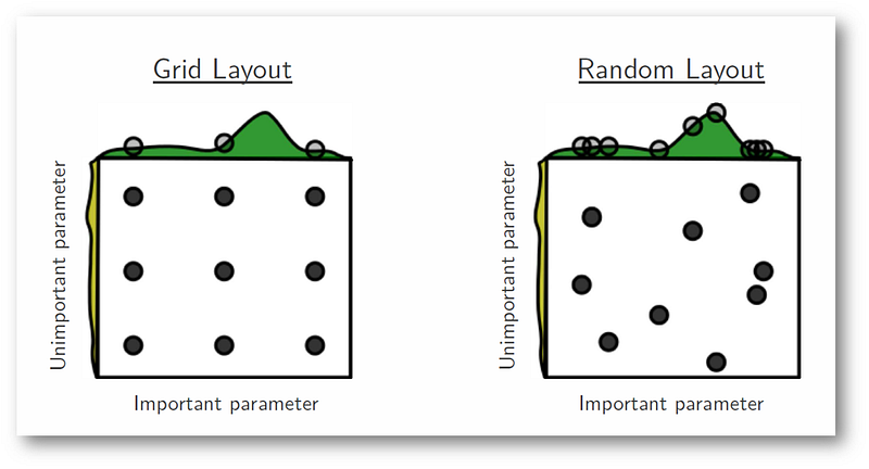
- Полный перебор (Grid Search) - явно задаются все возможные значения параметров. Далее перебираются все возможные комбинации этих параметров
- Случайный перебор (Random Search) - для некоотрых параметров задается распределение через функцию распределения. Задается количество случайных комбинаций, которых требуется перебрать.
- "Умный" перебор (hyperopt) - после каждого шага, следующия комбинация выбирается специальным образом, чтобы с одной стороны проверить неисследованные области, а с другой минимизировать функцию потерь. Не всегда работат так хорошо, как звучит.
Мы же попробует случайный поиск. Почему случайный поиск лучше перебора:
Задание
- С помощью GridSearchCV или RandomSearchCV подберите наиболее оптимальные параметры для случайного леса.
- Для этих параметров сравните средние результаты по кросс-валидации и качество на контрольной выборке
from sklearn.model_selection import GridSearchCV
from sklearn.model_selection import RandomizedSearchCV
# Your Code Here
from scipy.stats import randint as randint
from scipy.stats import uniform

try:
    from sklearn.model_selection import GridSearchCV
    from sklearn.model_selection import RandomizedSearchCV
    from sklearn.model_selection import StratifiedKFold
except ImportError:
    from sklearn.cross_validation import GridSearchCV
    from sklearn.cross_validation import RandomizedSearchCV
    from sklearn.cross_validation import StratifiedKFold


RND_SEED = 123
# Определим пространство поиска

param_grid = {
    'criterion': ['gini', 'entropy'],
    'max_depth': randint(2, 10),
    'min_samples_leaf': randint(1, 100),
    'class_weight': [None, 'balanced']}

# Некоторые параметры мы задали не простым перечислением значений, а
# с помощью распределений.

# Будем делать 200 запусков поиска
cv = StratifiedKFold(n_splits=5, random_state=123, shuffle=True)

model = DecisionTreeClassifier(random_state=123)
random_search = RandomizedSearchCV(model, param_distributions=param_grid, n_iter=200, n_jobs=-1,
                                   cv=cv, scoring='roc_auc', random_state=123)
# А дальше, просто .fit()
random_search.fit(X, y)
RandomizedSearchCV(cv=StratifiedKFold(n_splits=5, random_state=123, shuffle=True),
          error_score='raise-deprecating',
          estimator=DecisionTreeClassifier(class_weight=None, criterion='gini', max_depth=None,
            max_features=None, max_leaf_nodes=None,
            min_impurity_decrease=0.0, min_impurity_split=None,
            min_samples_leaf=1, min_samples_split=2,
            min_weight_fraction_leaf=0.0, presort=False, random_state=123,
            splitter='best'),
          fit_params=None, iid='warn', n_iter=200, n_jobs=-1,
          param_distributions={'criterion': ['gini', 'entropy'], 'max_depth': <scipy.stats._distn_infrastructure.rv_frozen object at 0x1a19606ba8>, 'min_samples_leaf': <scipy.stats._distn_infrastructure.rv_frozen object at 0x1a19ca73c8>, 'class_weight': [None, 'balanced']},
          pre_dispatch='2*n_jobs', random_state=123, refit=True,
          return_train_score='warn', scoring='roc_auc', verbose=0)
random_search.best_estimator_
DecisionTreeClassifier(class_weight=None, criterion='gini', max_depth=8,
            max_features=None, max_leaf_nodes=None,
            min_impurity_decrease=0.0, min_impurity_split=None,
            min_samples_leaf=95, min_samples_split=2,
            min_weight_fraction_leaf=0.0, presort=False, random_state=123,
            splitter='best')
random_search.best_score_
0.6135310935440562
random_search.best_params_
{'class_weight': None,
 'criterion': 'gini',
 'max_depth': 8,
 'min_samples_leaf': 95}