import pandas as pd
import numpy as np
import matplotlib.pyplot as plt

%matplotlib inline

plt.style.use('ggplot')
plt.rcParams['figure.figsize'] = (12,5)

# Для кириллицы на графиках
font = {'family': 'Verdana',
        'weight': 'normal'}
plt.rc('font', **font)

try:
    from ipywidgets import interact, IntSlider, fixed, FloatSlider
except ImportError:
    print(u'Так надо')
Вспоминаем про линейные модели
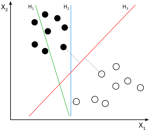
Уравнение прямой задаётся как: $$g(x) = w_0 + w_1x_1 + w_2x_2 = w_0 + \langle w, x \rangle = w_0 + w^\top x $$
- Если $g(x^*) > 0$, то $y^* = \text{'черный'} = +1$
- Если $g(x^*) < 0$, то $y^* = \text{'белый'} = -1$
- Если $g(x^*) = 0$, то мы находимся на линии
- т.е. решающее правило: $y^* = sign(g(x^*))$
Некоторые геометрические особенности
- $\frac{|g(x)|}{||w||}$ - расстояние от точки $x$ до гиперплоскости, степень "уверенности" в классификациий
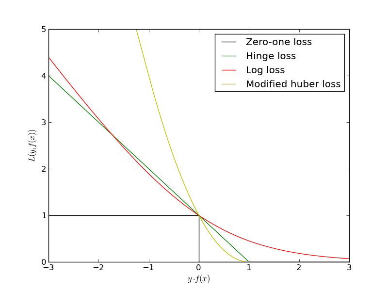
- Величину $M = y(\langle w, x \rangle + w_0) = y \cdot g(x)$ называют отступом(margin)
Если для какого-то объекта $x_i$ его отступ $M_i \geq 0$, то его классификация выполнена успешно.
Линейноразделимый случай с двумя классами
- Заметим что $g(x) = w_0 + \langle w, x \rangle$ и $g'(x) = c \cdot (w_0 + \langle w, x \rangle)$, $\forall c>0$ задают одну и ту же гиперплоскость
- Подберем $c$ таким образом, чтобы $\min\limits_i M_i = \min\limits_i y^{(i)} \cdot g(x^{(i)}) = 1$
- Объекты $x^{(i)}$ для которых $M^*_i = 1$ будем называть опорными

- Разделяющая полоса: $ -1 \leq w_0 + \langle w, x \rangle \leq +1$
- Ширина разделяющей полосы:
$$\langle (x^{+} - x^{-}) , \frac{w}{||w||}\rangle = \frac{\langle w, x^{+} \rangle - \langle w, x^{-} \rangle }{||w||} = \frac{2}{||w||} \rightarrow \max$$
- Таким образом мы придем к оптимизационной задаче:
from sklearn.datasets.samples_generator import make_classification

from sklearn.svm import SVC
from sklearn.linear_model import LogisticRegression

def plot_svc_decision_function(clf1, ax=None):
    if ax is None:
        ax = plt.gca()
    x = np.linspace(plt.xlim()[0], plt.xlim()[1], 30)
    y = np.linspace(plt.ylim()[0], plt.ylim()[1], 30)
    XX, YY = np.meshgrid(x, y)
    XY = np.c_[XX.ravel(), YY.ravel()]
    P1 = clf1.decision_function(XY)
    P1 = P1.reshape(XX.shape)

    # plot the margins
    cplot = ax.contour(XX, YY, P1, colors='k', label='svm',
               levels=[-1, 0, 1], alpha=0.5,
               linestyles=['--', '-', '--'])
    ax.clabel(cplot, inline=1, fontsize=10)
class_sep = 1.4

X, y = make_classification(n_samples=100, n_features=2, n_informative=2, class_sep=class_sep, scale=1,
                           n_redundant=0, n_clusters_per_class=1, random_state=31)

lin_svm = SVC(kernel='linear', C=100).fit(X, y)

# Plotting the splitting hyperplane and support vectors
plt.figure(figsize=(10,7))
plt.scatter(X[:, 0], X[:, 1], c=y, s=70, cmap='autumn')
plot_svc_decision_function(lin_svm)
plt.scatter(lin_svm.support_vectors_[:, 0], lin_svm.support_vectors_[:, 1],
            s=200, facecolors='none')

plt.xlabel('$x_1$')
plt.ylabel('$x_2$')

plt.xlim(-1, 5)
plt.ylim(-3, 4)
(-3, 4)

print(lin_svm.coef_) # w1, w2

print(lin_svm.coef0) # w0
[[ 0.50589936  1.36629804]]
0.0
lin_svm.support_vectors_ # Координаты опорных векторов
lin_svm.support_ # индексы опорных векторов в X
array([10, 41, 54], dtype=int32)
# lin_svm.predict_proba(X) #SVM не умеет предсказывать вероятности
y_hat = lin_svm.predict(X) # метка класса
y_hat[:10]
array([0, 1, 1, 0, 1, 0, 1, 0, 0, 0])
y_hat_score = lin_svm.decision_function(X)
# "Расстояние" от
# гиперплоскости до объекта
y_hat_score[:10]
array([-5.36885256,  2.61733817,  2.44638215, -3.34662808,  1.49461987,
       -1.94482004,  1.62022006, -2.22515071, -4.18415577, -4.00759831])
Неразделимый случай
Будем допускать пропуск объектов за разделительную линию
- Вместо условия $y^{(i)}(\langle w, x^{(i)} \rangle + w_0 ) \geq 1$
- Будет условие $y^{(i)}(\langle w, x^{(i)} \rangle + w_0 ) \geq 1 - \xi_i, \quad \xi_i \geq 0$

А целевой функционал заменим на
$$ \frac{1}{2} ||w||^2 + C\sum\limits_i\xi_i \rightarrow \min\limits_{w,w_0,\xi} $$Таким образом мы придем к оптимизационной задаче: $$ \begin{cases} \frac{1}{2} ||w||^2 + C\sum\limits_i\xi_i \rightarrow \min\limits_{w,w_0,\xi} \\ y^{(i)}(\langle w, x^{(i)} \rangle + w_0 ) \geq 1 - \xi_i \quad i=1\dots n \\ \xi_i \geq 0 \quad i=1\dots n \end{cases} $$
class_sep = 1.4

X, y = make_classification(n_samples=100, n_features=2, n_informative=2, class_sep=class_sep, scale=1,
                           n_redundant=0, n_clusters_per_class=1, random_state=31)

lin_svm = SVC(kernel='linear', C=0.1).fit(X, y)

# Plotting the splitting hyperplane and support vectors
plt.figure(figsize=(10,7))
plt.scatter(X[:, 0], X[:, 1], c=y, s=70, cmap='autumn')
plot_svc_decision_function(lin_svm)
plt.scatter(lin_svm.support_vectors_[:, 0], lin_svm.support_vectors_[:, 1],
            s=200, facecolors='none')

plt.xlabel('$x_1$')
plt.ylabel('$x_2$')

plt.xlim(-1, 5)
plt.ylim(-3, 4)
(-3, 4)

Ядра и спрямляющие пространства

from sklearn.datasets.samples_generator import make_circles
from mpl_toolkits import mplot3d

X, y = make_circles(n_samples=100, factor=0.1,
                    noise=0.1, random_state=0)

fig = plt.figure()
ax = fig.add_subplot(1, 2, 1)

ax.scatter(X[:, 0], X[:, 1], c=y, s=70, cmap='autumn')
ax.set_xlabel('$x_1$')
ax.set_ylabel('$x_2$')

r = X[:, 0] ** 2 + X[:, 1] ** 2

ax = fig.add_subplot(1, 2, 2)

ax = fig.add_subplot(1, 2, 2, projection='3d')
ax.scatter3D(X[:, 0], X[:, 1], r, c=y, s=70, cmap='autumn')
ax.view_init(elev=30, azim=30)
ax.set_xlabel('$x_1$')
ax.set_ylabel('$x_2$')
ax.set_zlabel('$x_1^2 + x_2^2$')
<matplotlib.text.Text at 0x114023c90>

- $\psi: X \rightarrow H$
- $H$ - пространство большей размерности, в котором классы становятся линейноразделимыми называется спрямляющим.
- Разделяющся гиперплоскость в таком пространстве будет линейной, но при проекции на исходное пространство $X$ - нет
Представим, что мы как-то перешли в спрямляющее пространство и хотим строить SVM там? Что изменится в задаче оптимизации?
Наиболее популярны следующие ядра:
- Линейное (linear): $$\langle x, y\rangle$$
- Полиномиальное (polynomial): $$(\gamma \langle x, y\rangle + с)^d,$$
- Radial basis function kernel (rbf): $$e^{(-\gamma \cdot \|x - y\|^2)},$$
- Sigmoid: $$\tanh(\gamma \langle x,y \rangle + r)$$
from IPython.display import YouTubeVideo
YouTubeVideo('3liCbRZPrZA', width=640, height=480)
class_sep = 1.4

X, y = make_circles(n_samples=100, factor=0.1,
                    noise=0.1, random_state=0)

lin_svm = SVC(kernel='rbf', C=1.0, gamma=60).fit(X, y)

# Plotting the splitting hyperplane and support vectors
plt.figure(figsize=(10,7))
plt.scatter(X[:, 0], X[:, 1], c=y, s=70, cmap='autumn')
plot_svc_decision_function(lin_svm)
plt.scatter(lin_svm.support_vectors_[:, 0], lin_svm.support_vectors_[:, 1],
            s=200, facecolors='none')

plt.xlabel('$x_1$')
plt.ylabel('$x_2$')

plt.xlim(-1, 1)
plt.ylim(-1, 1)
(-1, 1)

Метод опорных векторов для регрессии?
Практика
Загрузите текстовые данные отсюда. Архив должен содержать 3 файла с положительными и отрицательными отзывами с ресурсов
- imdb.com
- amazon.com
- yelp.com
Формат файла следующий: <отзыв>\t<метка>\n
Задача
- Загрузите тексты и метки классов в разные переменные
- Выберите меру качества классификации
- Обучите линейный SVM (без подбора гиперпараметров). Тексты представляются в виде мешка слов
- Выведите наиболее значимые слова из текста
- С помощью кросс-валидации и валидационных кривых исследуйте, как различные комбинции параметров влияют на качество
!ls ./sentiment\ labelled\ sentences
amazon_cells_labelled.txt readme.txt
imdb_labelled.txt         yelp_labelled.txt
texts, labels = [], []

for line in open('./sentiment labelled sentences/amazon_cells_labelled.txt'):
    text, label = line.strip('\n').split('\t')
    texts.append(text)
    labels.append(int(label))
from sklearn.feature_extraction.text import TfidfVectorizer
from sklearn.pipeline import Pipeline

model = Pipeline(
[
    ('vect', TfidfVectorizer()),
    ('svm', SVC(kernel='linear'))
])
model.fit(texts, labels)
Pipeline(steps=[('vect', TfidfVectorizer(analyzer=u'word', binary=False, decode_error=u'strict',
        dtype=<type 'numpy.int64'>, encoding=u'utf-8', input=u'content',
        lowercase=True, max_df=1.0, max_features=None, min_df=1,
        ngram_range=(1, 1), norm=u'l2', preprocessor=None, smooth_idf=True...,
  max_iter=-1, probability=False, random_state=None, shrinking=True,
  tol=0.001, verbose=False))])
weights = model.steps[1][1].coef_.toarray()[0]
words = model.steps[0][1].get_feature_names()
coefs = pd.Series(index=words, data=weights)
coefs.sort_values()
not             -3.507181
first           -1.975821
poor            -1.965497
doesn           -1.505776
bad             -1.485459
if              -1.456254
none            -1.446073
difficult       -1.376058
disappointed    -1.374236
then            -1.372565
unreliable      -1.359178
old             -1.344775
worst           -1.294790
disappointing   -1.292949
terrible        -1.290509
hear            -1.255339
money           -1.162993
however         -1.148374
don             -1.145519
horrible        -1.063185
problem         -1.036764
within          -1.013970
return          -1.007565
waste           -1.005096
stay            -1.003578
buying          -0.996052
sucks           -0.976878
experience      -0.958927
off             -0.953516
crap            -0.947778
                   ...
all              1.077599
car              1.091398
rocks            1.125765
happy            1.163118
awesome          1.169940
beautiful        1.170902
any              1.173849
seems            1.181771
setup            1.185614
definitely       1.194722
worthwhile       1.198160
pleased          1.216341
exactly          1.236538
and              1.242878
sturdy           1.324035
glad             1.324793
perfectly        1.472077
without          1.489238
comfortable      1.565059
well             1.579040
recommend        1.776462
than             1.781467
easy             1.834265
excellent        1.876684
nice             1.923456
love             1.954578
works            2.188037
best             2.503786
good             2.569317
great            3.112906
dtype: float64