Time-varying frame
Renato Naville Watanabe, Marcos Duarte
Laboratory of Biomechanics and Motor Control
Federal University of ABC, Brazil
Python setup
import numpy as np
import sympy as sym
from sympy.vector import CoordSys3D
import matplotlib.pyplot as plt
sym.init_printing()
from sympy.plotting import plot_parametric
from sympy.physics.mechanics import ReferenceFrame, Vector, dot
from matplotlib.patches import FancyArrowPatch
plt.rcParams.update({'figure.figsize':(8, 5), 'lines.linewidth':2})
Cartesian coordinate system
As we perceive the surrounding space as three-dimensional, a convenient coordinate system is the Cartesian coordinate system in the Euclidean space with three orthogonal axes as shown below. The axes directions are commonly defined by the right-hand rule and attributed the letters X, Y, Z. The orthogonality of the Cartesian coordinate system is convenient for its use in classical mechanics, most of the times the structure of space is assumed having the Euclidean geometry and as consequence, the motion in different directions are independent of each other.

Determination of a coordinate system
In Biomechanics, we may use different coordinate systems for convenience and refer to them as global, laboratory, local, anatomical, or technical reference frames or coordinate systems.
From linear algebra, a set of unit linearly independent vectors (orthogonal in the Euclidean space and each with norm (length) equals to one) that can represent any vector via linear combination is called a basis (or orthonormal basis). The figure below shows a point and its position vector in the Cartesian coordinate system and the corresponding versors (unit vectors) of the basis for this coordinate system. See the notebook Scalar and vector for a description on vectors.

One can see that the versors of the basis shown in the figure above have the following coordinates in the Cartesian coordinate system:
\begin{equation} \hat{\mathbf{i}} = \begin{bmatrix}1\\0\\0 \end{bmatrix}, \quad \hat{\mathbf{j}} = \begin{bmatrix}0\\1\\0 \end{bmatrix}, \quad \hat{\mathbf{k}} = \begin{bmatrix} 0 \\ 0 \\ 1 \end{bmatrix} \label{eq_1} \end{equation}
Using the notation described in the figure above, the position vector $\overrightarrow{\mathbf{r}}$ can be expressed as:
\begin{equation} \overrightarrow{\mathbf{r}} = x\hat{\mathbf{i}} + y\hat{\mathbf{j}} + z\hat{\mathbf{k}} \label{eq_2} \end{equation}
However, to use a fixed basis can lead to very complex expressions.
Time varying basis
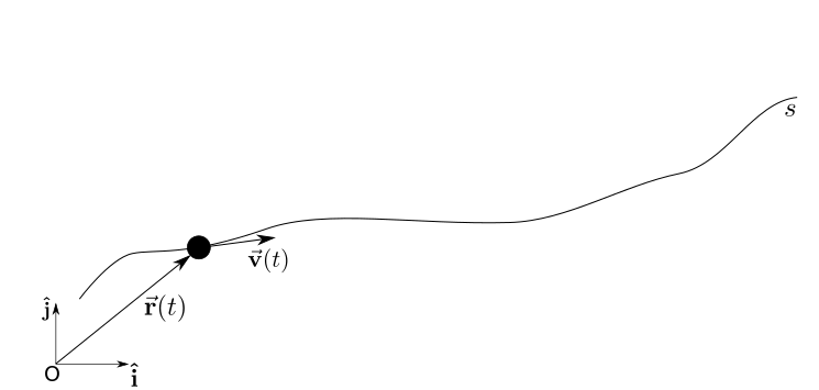
Consider that we have the position vector of a particle, moving in the path described by the parametric curve $s(t)$, described in a fixed reference frame as:
\begin{equation} {\bf\hat{r}}(t) = {x}{\bf\hat{i}}+{y}{\bf\hat{j}} + {z}{\bf\hat{k}} \label{eq_3} \end{equation}
Tangential versor
Often we describe all the kinematic variables in this fixed reference frame. However, it is often useful to define a time-varying basis, attached to some point of interest. In this case, what is usually done is to choose as one of the basis vector a unitary vector in the direction of the velocity of the particle. Defining this vector as:
\begin{equation} {\bf\hat{e}_t} = \frac{{\bf\vec{v}}}{\Vert{\bf\vec{v}}\Vert} \label{eq_4} \end{equation}Normal versor
For the second vector of the basis, we define first a vector of curvature of the path (the meaning of this curvature vector will be seeing in another notebook):
\begin{equation} {\bf\vec{C}} = \frac{d{\bf\hat{e}_t}}{ds} \label{eq_5} \end{equation}
Note that $\bf\hat{e}_t$ is a function of the path $s(t)$. So, by the chain rule:
\begin{equation} \frac{d{\bf\hat{e}_t}}{dt} = \frac{d{\bf\hat{e}_t}}{ds}\frac{ds}{dt} \longrightarrow \frac{d{\bf\hat{e}_t}}{ds} = \frac{\frac{d{\bf\hat{e}_t}}{dt}}{\frac{ds}{dt}} \longrightarrow {\bf\vec{C}} = \frac{\frac{d{\bf\hat{e}_t}}{dt}}{\frac{ds}{dt}}\longrightarrow {\bf\vec{C}} = \frac{\frac{d{\bf\hat{e}_t}}{dt}}{\Vert{\bf\vec{v}}\Vert} \label{eq_6} \end{equation}
Now we can define the second vector of the basis, ${\bf\hat{e}_n}$:
\begin{equation} {\bf\hat{e}_n} = \frac{{\bf\vec{C}}}{\Vert{\bf\vec{C}}\Vert} \label{eq_7} \end{equation}

Binormal versor
The third vector of the basis is obtained by the cross product between ${\bf\hat{e}_n}$ and ${\bf\hat{e}_t}$:
\begin{equation} {\bf\hat{e}_b} = {\bf\hat{e}_t} \times {\bf\hat{e}_n} \label{eq_8} \end{equation}
Note that the vectors ${\bf\hat{e}_t}$ , ${\bf\hat{e}_n}$ and ${\bf\hat{e}_b}$ vary together with the particle movement.
Velocity and Acceleration in a time-varying frame
Velocity
Given the expression of $r(t)$ in a fixed frame we can write the velocity ${\bf\vec{v}(t)}$ as a function of the fixed frame of reference ${\bf\hat{i}}$, ${\bf\hat{j}}$ and ${\bf\hat{k}}$ (see http://nbviewer.jupyter.org/github/BMClab/bmc/blob/master/notebooks/KinematicsParticle.ipynb)).
\begin{equation} {\bf\vec{v}}(t) = \dot{x}{\bf\hat{i}}+\dot{y}{\bf\hat{j}}+\dot{z}{\bf\hat{k}} \label{eq_9} \end{equation}
However, this can lead to very complex functions. So it is useful to use the basis find previously ${\bf\hat{e}_t}$, ${\bf\hat{e}_n}$ and ${\bf\hat{e}_b}$.
The velocity ${\bf\vec{v}}$ of the particle is, by the definition of ${\bf\hat{e}_t}$, in the direction of ${\bf\hat{e}_t}$:
\begin{equation} {\bf\vec{v}}={\Vert\bf\vec{v}\Vert}.{\bf\hat{e}_t} \label{eq_10} \end{equation}
Acceleration
The acceleration can be written in the fixed frame of reference as:
\begin{equation} {\bf\vec{a}}(t) = \ddot{x}{\bf\hat{i}}+\ddot{y}{\bf\hat{j}}+\ddot{z}{\bf\hat{k}} \label{eq_11} \end{equation}
But for the same reasons of the velocity vector, it is useful to describe the acceleration vector in the time varying basis. We know that the acceleration is the time derivative of the velocity:
\begin{align} {\bf\vec{a}} =& \frac{{d\bf\vec{v}}}{dt}=\\ =&\frac{{d({\Vert\bf\vec{v}\Vert}{\bf\hat{e}_t}})}{dt}=\\ =&\dot{\Vert\bf\vec{v}\Vert}{\bf\hat{e}_t}+{\Vert\bf\vec{v}\Vert}\dot{{\bf\hat{e}_t}}=\\ =&\dot{\Vert\bf\vec{v}\Vert}{\bf\hat{e}_t}+{\Vert\bf\vec{v}\Vert}\frac{d{\bf\hat{e}_t}}{ds}\frac{ds}{dt}=\\ =&\dot{\Vert\bf\vec{v}\Vert}{\bf\hat{e}_t}+{\Vert\bf\vec{v}\Vert}^2\frac{d{\bf\hat{e}_t}}{ds}=\\ =&\dot{\Vert\bf\vec{v}\Vert}{\bf\hat{e}_t}+{\Vert\bf\vec{v}\Vert}^2\Vert{\bf\vec{C}} \Vert {\bf\hat{e}_n} \label{eq_12} \end{align}
Example
For example, consider that a particle follows the path described by the parametric curve below:
\begin{equation} {\bf\vec{r}(t)} = (10t+100){\bf{\hat{i}}} + \left(-\frac{9,81}{2}t^2+50t+100\right){\bf{\hat{j}}} \label{eq_13} \end{equation}
This curve could be, for example, from a projectile motion. See http://nbviewer.jupyter.org/github/BMClab/bmc/blob/master/notebooks/ProjectileMotion.ipynb for an explanation on projectile motion.
Solving numerically
Now we will obtain the time-varying basis numerically. This method is useful when it is not available a mathematical expression of the path. This often happens when you have available data collected experimentally (most of the cases in Biomechanics).
First, data will be obtained from the expression of $r(t)$. This is done to replicate the example above. You could use data collected experimentally, for example.
t = np.linspace(0, 10, 1000).reshape(-1,1)
r = np.hstack((10*t + 100, -9.81/2*t**2 + 50*t + 100))
Now, to obtain the $\bf{\hat{e_t}}$ versor, we can use Equation (4).
dt = t[1]
v = np.diff(r,axis=0)/dt
vNorm  = np.linalg.norm(v, axis=1, keepdims=True)

et = v/vNorm
And to obtain the versor $\bf{\hat{e_n}}$, we can use Equation (8).
C = np.diff(et,axis=0)/dt
C = C/vNorm[1:]

CNorm = np.linalg.norm(C, axis=1, keepdims=True)
en = C/CNorm
fig = plt.figure()
plt.plot(r[:, 0], r[:, 1], '.')
ax = fig.add_axes([0, 0, 1, 1])
time = np.linspace(0, 10, 10)
for i in np.arange(0, len(t)-2, 50):
    vec1 = FancyArrowPatch(r[i, :], r[i, :]+10*et[i, :], mutation_scale=20, color='r')
    vec2 = FancyArrowPatch(r[i, :], r[i, :]+10*en[i, :], mutation_scale=20, color='g')
    ax.add_artist(vec1)
    ax.add_artist(vec2)
plt.xlim((80, 250))
plt.ylim((80, 250))
plt.legend([vec1, vec2], [r'$\vec{e_t}$', r'$\vec{e_{n}}$'])
plt.show()

v  = vNorm*et
vNormDot  = np.diff(vNorm, axis=0)/dt

a = vNormDot*et[1:,:] + CNorm*en*vNorm[1:]**2
fig = plt.figure()
plt.plot(r[:, 0], r[:, 1], '.')
ax = fig.add_axes([0, 0, 1, 1])
for i in range(0, len(t)-2, 50):
    vec1 = FancyArrowPatch(r[i, :], r[i, :]+v[i, :], mutation_scale=10, color='r')
    vec2 = FancyArrowPatch(r[i, :], r[i, :]+a[i, :], mutation_scale=10, color='g')
    ax.add_artist(vec1)
    ax.add_artist(vec2)
plt.xlim((80, 250))
plt.ylim((80, 250))
plt.legend([vec1, vec2], [r'$\vec{v}$', r'$\vec{a}$'])
plt.show()

Symbolic solution (extra reading)
The computation here will be performed symbolically, with the symbolic math package of Python, Sympy. Below,a reference frame, called O, and a varible for time (t) are defined.
O = sym.vector.CoordSys3D(' ')
t = sym.symbols('t')
Below the vector $r(t)$ is defined symbolically.
r = (10*t+100)*O.i + (-9.81/2*t**2+50*t+100)*O.j+0*O.k
r
p1 = plot_parametric(r.dot(O.i), r.dot(O.j), (t, 0, 10), line_width=4, aspect_ratio=(2, 1))

v = sym.diff(r)
v
et = v/sym.sqrt(v.dot(v))
et
C = sym.diff(et)/sym.sqrt(v.dot(v))
C
en = C/(sym.sqrt(C.dot(C)))
sym.simplify(en)
fig = plt.figure()
ax = fig.add_axes([0, 0, 1, 1])
time = np.linspace(0, 10, 30)
for instant in time:
    vt = FancyArrowPatch([float(r.dot(O.i).subs(t,instant)),float(r.dot(O.j).subs(t,instant))],
                         [float(r.dot(O.i).subs(t,instant))+10*float(et.dot(O.i).subs(t,instant)),
                          float(r.dot(O.j).subs(t, instant))+10*float(et.dot(O.j).subs(t,instant))],
                         mutation_scale=20,
                         arrowstyle="->",color="r",label='${\hat{e_t}}$', lw=2)
    vn = FancyArrowPatch([float(r.dot(O.i).subs(t, instant)),float(r.dot(O.j).subs(t,instant))],
                         [float(r.dot(O.i).subs(t, instant))+10*float(en.dot(O.i).subs(t, instant)),
                          float(r.dot(O.j).subs(t, instant))+10*float(en.dot(O.j).subs(t, instant))],
                         mutation_scale=20,
                         arrowstyle="->",color="g",label='${\hat{e_n}}$', lw=2)
    ax.add_artist(vn)
    ax.add_artist(vt)
plt.xlim((90, 250))
plt.ylim((90, 250))
plt.xlabel('x')
plt.legend(handles=[vt, vn], fontsize=20)
plt.show()

Now we can find the vectors ${\bf\vec{v}}$ and ${\bf\vec{a}}$ described in the time varying frame.
v = sym.sqrt(v.dot(v))*et
a = sym.diff(sym.sqrt(v.dot(v)))*et+v.dot(v)*sym.sqrt(C.dot(C))*en
sym.simplify(sym.simplify(a))
fig = plt.figure()
ax = fig.add_axes([0, 0, 1, 1])
time = np.linspace(0, 10, 10)
for instant in time:
    vt = FancyArrowPatch([float(r.dot(O.i).subs(t,instant)),float(r.dot(O.j).subs(t,instant))],
                         [float(r.dot(O.i).subs(t,instant))+float(v.dot(O.i).subs(t,instant)),
                          float(r.dot(O.j).subs(t, instant))+float(v.dot(O.j).subs(t,instant))],
                         mutation_scale=20,
                         arrowstyle="->",color="r",label='${{v}}$', lw=2)
    vn = FancyArrowPatch([float(r.dot(O.i).subs(t, instant)),float(r.dot(O.j).subs(t,instant))],
                         [float(r.dot(O.i).subs(t, instant))+float(a.dot(O.i).subs(t, instant)),
                          float(r.dot(O.j).subs(t, instant))+float(a.dot(O.j).subs(t, instant))],
                         mutation_scale=20,
                         arrowstyle="->",color="g",label='${{a}}$', lw=2)
    ax.add_artist(vn)
    ax.add_artist(vt)
plt.xlim((60, 250))
plt.ylim((60, 250))
plt.legend(handles=[vt, vn], fontsize=20)
plt.show()

Further Reading
- Read pages 932-971 of the 18th chapter of the Ruina and Rudra's book about time-varying basis vectors.
Video lectures on the Internet
Problems
- Obtain the vectors $\hat{e_n}$ and $\hat{e_t}$ for the problem 17.1.1 from Ruina and Rudra's book.
- Solve the problem 17.1.9 from Ruina and Rudra's book.
- Write a Python program to solve the problem 17.1.10 (only the part of $\hat{e_n}$ and $\hat{e_t}$).
- A particle has its position vector along time equal to ${\bf\vec{r}(t)} = R\cos(\omega t){\bf\hat{i}} + R\sin(\omega t){\bf\hat{j}}$. Find the curvature vector ${\bf\vec{C}}$ as a function of time. Draw the vector ${\bf\vec{C}}$ at some points of the particle path.
References
- Ruina A, Rudra P (2019) Introduction to Mechanics for Engineers. Oxford University Press.