Generative Adversarial Networks (GANs)
So far in CS231N, all the applications of neural networks that we have explored have been discriminative models that take an input and are trained to produce a labeled output. This has ranged from straightforward classification of image categories to sentence generation (which was still phrased as a classification problem, our labels were in vocabulary space and we’d learned a recurrence to capture multi-word labels). In this notebook, we will expand our repetoire, and build generative models using neural networks. Specifically, we will learn how to build models which generate novel images that resemble a set of training images.
What is a GAN?
In 2014, Goodfellow et al. presented a method for training generative models called Generative Adversarial Networks (GANs for short). In a GAN, we build two different neural networks. Our first network is a traditional classification network, called the discriminator. We will train the discriminator to take images, and classify them as being real (belonging to the training set) or fake (not present in the training set). Our other network, called the generator, will take random noise as input and transform it using a neural network to produce images. The goal of the generator is to fool the discriminator into thinking the images it produced are real.
We can think of this back and forth process of the generator ($G$) trying to fool the discriminator ($D$), and the discriminator trying to correctly classify real vs. fake as a minimax game: $$\underset{G}{\text{minimize}}\; \underset{D}{\text{maximize}}\; \mathbb{E}_{x \sim p_\text{data}}\left[\log D(x)\right] + \mathbb{E}_{z \sim p(z)}\left[\log \left(1-D(G(z))\right)\right]$$ where $x \sim p_\text{data}$ are samples from the input data, $z \sim p(z)$ are the random noise samples, $G(z)$ are the generated images using the neural network generator $G$, and $D$ is the output of the discriminator, specifying the probability of an input being real. In Goodfellow et al., they analyze this minimax game and show how it relates to minimizing the Jensen-Shannon divergence between the training data distribution and the generated samples from $G$.
To optimize this minimax game, we will aternate between taking gradient descent steps on the objective for $G$, and gradient ascent steps on the objective for $D$:
- update the generator ($G$) to minimize the probability of the discriminator making the correct choice.
- update the discriminator ($D$) to maximize the probability of the discriminator making the correct choice.
While these updates are useful for analysis, they do not perform well in practice. Instead, we will use a different objective when we update the generator: maximize the probability of the discriminator making the incorrect choice. This small change helps to allevaiate problems with the generator gradient vanishing when the discriminator is confident. This is the standard update used in most GAN papers, and was used in the original paper from Goodfellow et al..
In this assignment, we will alternate the following updates:
- Update the generator ($G$) to maximize the probability of the discriminator making the incorrect choice on generated data:
- Update the discriminator ($D$), to maximize the probability of the discriminator making the correct choice on real and generated data:
What else is there?
Since 2014, GANs have exploded into a huge research area, with massive workshops, and hundreds of new papers. Compared to other approaches for generative models, they often produce the highest quality samples but are some of the most difficult and finicky models to train (see this github repo that contains a set of 17 hacks that are useful for getting models working). Improving the stabiilty and robustness of GAN training is an open research question, with new papers coming out every day! For a more recent tutorial on GANs, see here. There is also some even more recent exciting work that changes the objective function to Wasserstein distance and yields much more stable results across model architectures: WGAN, WGAN-GP.
GANs are not the only way to train a generative model! For other approaches to generative modeling check out the deep generative model chapter of the Deep Learning book. Another popular way of training neural networks as generative models is Variational Autoencoders (co-discovered here and here). Variational autoencoders combine neural networks with variational inference to train deep generative models. These models tend to be far more stable and easier to train but currently don't produce samples that are as pretty as GANs.
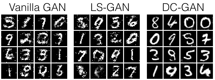
Example pictures of what you should expect (yours might look slightly different):
Setup
from __future__ import print_function, division
import tensorflow as tf
import numpy as np

import matplotlib.pyplot as plt
import matplotlib.gridspec as gridspec

%matplotlib inline
plt.rcParams['figure.figsize'] = (10.0, 8.0) # set default size of plots
plt.rcParams['image.interpolation'] = 'nearest'
plt.rcParams['image.cmap'] = 'gray'

# A bunch of utility functions

def show_images(images):
    images = np.reshape(images, [images.shape[0], -1])  # images reshape to (batch_size, D)
    sqrtn = int(np.ceil(np.sqrt(images.shape[0])))
    sqrtimg = int(np.ceil(np.sqrt(images.shape[1])))

    fig = plt.figure(figsize=(sqrtn, sqrtn))
    gs = gridspec.GridSpec(sqrtn, sqrtn)
    gs.update(wspace=0.05, hspace=0.05)

    for i, img in enumerate(images):
        ax = plt.subplot(gs[i])
        plt.axis('off')
        ax.set_xticklabels([])
        ax.set_yticklabels([])
        ax.set_aspect('equal')
        plt.imshow(img.reshape([sqrtimg,sqrtimg]))
    return

def preprocess_img(x):
    return 2 * x - 1.0

def deprocess_img(x):
    return (x + 1.0) / 2.0

def rel_error(x,y):
    return np.max(np.abs(x - y) / (np.maximum(1e-8, np.abs(x) + np.abs(y))))

def count_params():
    """Count the number of parameters in the current TensorFlow graph """
    param_count = np.sum([np.prod(x.get_shape().as_list()) for x in tf.global_variables()])
    return param_count


def get_session():
    config = tf.ConfigProto()
    config.gpu_options.allow_growth = True
    session = tf.Session(config=config)
    return session

answers = np.load('gan-checks-tf.npz')
Dataset
GANs are notoriously finicky with hyperparameters, and also require many training epochs. In order to make this assignment approachable without a GPU, we will be working on the MNIST dataset, which is 60,000 training and 10,000 test images. Each picture contains a centered image of white digit on black background (0 through 9). This was one of the first datasets used to train convolutional neural networks and it is fairly easy -- a standard CNN model can easily exceed 99% accuracy.
To simplify our code here, we will use the TensorFlow MNIST wrapper, which downloads and loads the MNIST dataset. See the documentation for more information about the interface. The default parameters will take 5,000 of the training examples and place them into a validation dataset. The data will be saved into a folder called MNIST_data.
Heads-up: The TensorFlow MNIST wrapper returns images as vectors. That is, they're size (batch, 784). If you want to treat them as images, we have to resize them to (batch,28,28) or (batch,28,28,1). They are also type np.float32 and bounded [0,1].
from tensorflow.examples.tutorials.mnist import input_data
mnist = input_data.read_data_sets('./cs231n/datasets/MNIST_data', one_hot=False)

# show a batch
show_images(mnist.train.next_batch(16)[0])
Extracting ./cs231n/datasets/MNIST_data/train-images-idx3-ubyte.gz
Extracting ./cs231n/datasets/MNIST_data/train-labels-idx1-ubyte.gz
Extracting ./cs231n/datasets/MNIST_data/t10k-images-idx3-ubyte.gz
Extracting ./cs231n/datasets/MNIST_data/t10k-labels-idx1-ubyte.gz

LeakyReLU
In the cell below, you should implement a LeakyReLU. See the class notes (where alpha is small number) or equation (3) in this paper. LeakyReLUs keep ReLU units from dying and are often used in GAN methods (as are maxout units, however those increase model size and therefore are not used in this notebook).
HINT: You should be able to use tf.maximum
def leaky_relu(x, alpha=0.01):
    """Compute the leaky ReLU activation function.

    Inputs:
    - x: TensorFlow Tensor with arbitrary shape
    - alpha: leak parameter for leaky ReLU

    Returns:
    TensorFlow Tensor with the same shape as x
    """
    # TODO: implement leaky ReLU
    x_leak = x*alpha
    y = tf.maximum(x, x_leak)
    return y
Test your leaky ReLU implementation. You should get errors < 1e-10
def test_leaky_relu(x, y_true):
    tf.reset_default_graph()
    with get_session() as sess:
        y_tf = leaky_relu(tf.constant(x))
        y = sess.run(y_tf)
        print('Maximum error: %g'%rel_error(y_true, y))

test_leaky_relu(answers['lrelu_x'], answers['lrelu_y'])
Maximum error: 0
Random Noise
Generate a TensorFlow Tensor containing uniform noise from -1 to 1 with shape [batch_size, dim].
def sample_noise(batch_size, dim):
    """Generate random uniform noise from -1 to 1.

    Inputs:
    - batch_size: integer giving the batch size of noise to generate
    - dim: integer giving the dimension of the the noise to generate

    Returns:
    TensorFlow Tensor containing uniform noise in [-1, 1] with shape [batch_size, dim]
    """
    # TODO: sample and return noise
    noise = tf.random_uniform([batch_size, dim], minval=-1, maxval=1)
    return noise
Make sure noise is the correct shape and type:
def test_sample_noise():
    batch_size = 3
    dim = 4
    tf.reset_default_graph()
    with get_session() as sess:
        z = sample_noise(batch_size, dim)
        # Check z has the correct shape
        assert z.get_shape().as_list() == [batch_size, dim]
        # Make sure z is a Tensor and not a numpy array
        assert isinstance(z, tf.Tensor)
        # Check that we get different noise for different evaluations
        z1 = sess.run(z)
        z2 = sess.run(z)
        assert not np.array_equal(z1, z2)
        # Check that we get the correct range
        assert np.all(z1 >= -1.0) and np.all(z1 <= 1.0)
        print("All tests passed!")

test_sample_noise()
All tests passed!
Discriminator
Our first step is to build a discriminator. You should use the layers in tf.layers to build the model.
All fully connected layers should include bias terms.
Architecture:
- Fully connected layer from size 784 to 256
- LeakyReLU with alpha 0.01
- Fully connected layer from 256 to 256
- LeakyReLU with alpha 0.01
- Fully connected layer from 256 to 1
The output of the discriminator should have shape [batch_size, 1], and contain real numbers corresponding to the scores that each of the batch_size inputs is a real image.
def discriminator(x):
    """Compute discriminator score for a batch of input images.

    Inputs:
    - x: TensorFlow Tensor of flattened input images, shape [batch_size, 784]

    Returns:
    TensorFlow Tensor with shape [batch_size, 1], containing the score
    for an image being real for each input image.
    """
    with tf.variable_scope("discriminator"):
        # TODO: implement architecture
        init = tf.contrib.layers.xavier_initializer(uniform=True)
        x = tf.layers.dense(x, 256, activation=leaky_relu, kernel_initializer=init, name='first_layer')
        x = tf.layers.dense(x, 256, activation=leaky_relu, kernel_initializer=init, name='second_layer')
        logits = tf.layers.dense(x, 1, kernel_initializer=init, name='logits')
        return logits
Test to make sure the number of parameters in the discriminator is correct:
def test_discriminator(true_count=267009):
    tf.reset_default_graph()
    with get_session() as sess:
        y = discriminator(tf.ones((2, 784)))
        cur_count = count_params()
        if cur_count != true_count:
            print('Incorrect number of parameters in discriminator. {0} instead of {1}. Check your achitecture.'.format(cur_count,true_count))
        else:
            print('Correct number of parameters in discriminator.')

test_discriminator()
Correct number of parameters in discriminator.
Generator
Now to build a generator. You should use the layers in tf.layers to construct the model. All fully connected layers should include bias terms.
Architecture:
- Fully connected layer from tf.shape(z)[1] (the number of noise dimensions) to 1024
- ReLU
- Fully connected layer from 1024 to 1024
- ReLU
- Fully connected layer from 1024 to 784
- TanH (To restrict the output to be [-1,1])
def generator(z):
    """Generate images from a random noise vector.

    Inputs:
    - z: TensorFlow Tensor of random noise with shape [batch_size, noise_dim]

    Returns:
    TensorFlow Tensor of generated images, with shape [batch_size, 784].
    """
    with tf.variable_scope("generator"):
        # TODO: implement architecture
        init = tf.contrib.layers.xavier_initializer(uniform=True)
        x = tf.layers.dense(z, 1024, activation=tf.nn.relu, kernel_initializer=init, name='first_layer')
        x = tf.layers.dense(x, 1024, activation=tf.nn.relu, kernel_initializer=init, name='second_layer')
        x = tf.layers.dense(x, 784, kernel_initializer=init, name='third_layer')
        img = tf.tanh(x, name='image')
        return img
Test to make sure the number of parameters in the generator is correct:
def test_generator(true_count=1858320):
    tf.reset_default_graph()
    with get_session() as sess:
        y = generator(tf.ones((1, 4)))
        cur_count = count_params()
        if cur_count != true_count:
            print('Incorrect number of parameters in generator. {0} instead of {1}. Check your achitecture.'.format(cur_count,true_count))
        else:
            print('Correct number of parameters in generator.')

test_generator()
Correct number of parameters in generator.
GAN Loss
Compute the generator and discriminator loss. The generator loss is: $$\ell_G = -\mathbb{E}_{z \sim p(z)}\left[\log D(G(z))\right]$$ and the discriminator loss is: $$ \ell_D = -\mathbb{E}_{x \sim p_\text{data}}\left[\log D(x)\right] - \mathbb{E}_{z \sim p(z)}\left[\log \left(1-D(G(z))\right)\right]$$ Note that these are negated from the equations presented earlier as we will be minimizing these losses.
HINTS: Use tf.ones_like and tf.zeros_like to generate labels for your discriminator. Use sigmoid_cross_entropy loss to help compute your loss function. Instead of computing the expectation, we will be averaging over elements of the minibatch, so make sure to combine the loss by averaging instead of summing.
def gan_loss(logits_real, logits_fake):
    """Compute the GAN loss.

    Inputs:
    - logits_real: Tensor, shape [batch_size, 1], output of discriminator
        Log probability that the image is real for each real image
    - logits_fake: Tensor, shape[batch_size, 1], output of discriminator
        Log probability that the image is real for each fake image

    Returns:
    - D_loss: discriminator loss scalar
    - G_loss: generator loss scalar
    """
    # TODO: compute D_loss and G_loss
    D_loss = tf.reduce_mean(tf.nn.sigmoid_cross_entropy_with_logits(
        labels=tf.ones_like(logits_real), logits=logits_real))+tf.reduce_mean(
        tf.nn.sigmoid_cross_entropy_with_logits(labels=tf.zeros_like(logits_fake),
        logits=logits_fake))
    G_loss = tf.reduce_mean(tf.nn.sigmoid_cross_entropy_with_logits(labels=tf.ones_like(logits_fake),
                                                                    logits=logits_fake))
    return D_loss, G_loss
Test your GAN loss. Make sure both the generator and discriminator loss are correct. You should see errors less than 1e-5.
def test_gan_loss(logits_real, logits_fake, d_loss_true, g_loss_true):
    tf.reset_default_graph()
    with get_session() as sess:
        d_loss, g_loss = sess.run(gan_loss(tf.constant(logits_real), tf.constant(logits_fake)))
    print("Maximum error in d_loss: %g"%rel_error(d_loss_true, d_loss))
    print("Maximum error in g_loss: %g"%rel_error(g_loss_true, g_loss))

test_gan_loss(answers['logits_real'], answers['logits_fake'],
              answers['d_loss_true'], answers['g_loss_true'])
Maximum error in d_loss: 0
Maximum error in g_loss: 0
Optimizing our loss
Make an AdamOptimizer with a 1e-3 learning rate, beta1=0.5 to mininize G_loss and D_loss separately. The trick of decreasing beta was shown to be effective in helping GANs converge in the Improved Techniques for Training GANs paper. In fact, with our current hyperparameters, if you set beta1 to the Tensorflow default of 0.9, there's a good chance your discriminator loss will go to zero and the generator will fail to learn entirely. In fact, this is a common failure mode in GANs; if your D(x) learns to be too fast (e.g. loss goes near zero), your G(z) is never able to learn. Often D(x) is trained with SGD with Momentum or RMSProp instead of Adam, but here we'll use Adam for both D(x) and G(z).
# TODO: create an AdamOptimizer for D_solver and G_solver
def get_solvers(learning_rate=1e-3, beta1=0.5):
    """Create solvers for GAN training.

    Inputs:
    - learning_rate: learning rate to use for both solvers
    - beta1: beta1 parameter for both solvers (first moment decay)

    Returns:
    - D_solver: instance of tf.train.AdamOptimizer with correct learning_rate and beta1
    - G_solver: instance of tf.train.AdamOptimizer with correct learning_rate and beta1
    """
    D_solver = tf.train.AdamOptimizer(learning_rate=learning_rate, beta1=beta1)
    G_solver = tf.train.AdamOptimizer(learning_rate=learning_rate, beta1=beta1)
    return D_solver, G_solver
Putting it all together
Now just a bit of Lego Construction. Read this section over carefully to understand how we'll be composing the generator and discriminator.
tf.reset_default_graph()

# number of images for each batch
batch_size = 128
# our noise dimension
noise_dim = 96

# placeholder for images from the training dataset
x = tf.placeholder(tf.float32, [None, 784])
# random noise fed into our generator
z = sample_noise(batch_size, noise_dim)
# generated images
G_sample = generator(z)

with tf.variable_scope("") as scope:
    #scale images to be -1 to 1
    logits_real = discriminator(preprocess_img(x))
    # Re-use discriminator weights on new inputs
    scope.reuse_variables()
    logits_fake = discriminator(G_sample)

# Get the list of variables for the discriminator and generator
D_vars = tf.get_collection(tf.GraphKeys.TRAINABLE_VARIABLES, 'discriminator')
G_vars = tf.get_collection(tf.GraphKeys.TRAINABLE_VARIABLES, 'generator')

# get our solver
D_solver, G_solver = get_solvers()

# get our loss
D_loss, G_loss = gan_loss(logits_real, logits_fake)

# setup training steps
D_train_step = D_solver.minimize(D_loss, var_list=D_vars)
G_train_step = G_solver.minimize(G_loss, var_list=G_vars)
D_extra_step = tf.get_collection(tf.GraphKeys.UPDATE_OPS, 'discriminator')
G_extra_step = tf.get_collection(tf.GraphKeys.UPDATE_OPS, 'generator')
Training a GAN!
Well that wasn't so hard, was it? In the iterations in the low 100s you should see black backgrounds, fuzzy shapes as you approach iteration 1000, and decent shapes, about half of which will be sharp and clearly recognizable as we pass 3000. In our case, we'll simply train D(x) and G(z) with one batch each every iteration. However, papers often experiment with different schedules of training D(x) and G(z), sometimes doing one for more steps than the other, or even training each one until the loss gets "good enough" and then switching to training the other.
# a giant helper function
def run_a_gan(sess, G_train_step, G_loss, D_train_step, D_loss, G_extra_step, D_extra_step,\
              show_every=250, print_every=50, batch_size=128, num_epoch=10):
    """Train a GAN for a certain number of epochs.

    Inputs:
    - sess: A tf.Session that we want to use to run our data
    - G_train_step: A training step for the Generator
    - G_loss: Generator loss
    - D_train_step: A training step for the Generator
    - D_loss: Discriminator loss
    - G_extra_step: A collection of tf.GraphKeys.UPDATE_OPS for generator
    - D_extra_step: A collection of tf.GraphKeys.UPDATE_OPS for discriminator
    Returns:
        Nothing
    """
    # compute the number of iterations we need
    max_iter = int(mnist.train.num_examples*num_epoch/batch_size)
    for it in range(max_iter):
        # every show often, show a sample result
        if it % show_every == 0:
            samples = sess.run(G_sample)
            fig = show_images(samples[:16])
            plt.show()
            print()
        # run a batch of data through the network
        minibatch,minbatch_y = mnist.train.next_batch(batch_size)
        _, D_loss_curr = sess.run([D_train_step, D_loss], feed_dict={x: minibatch})
        _, G_loss_curr = sess.run([G_train_step, G_loss])

        # print loss every so often.
        # We want to make sure D_loss doesn't go to 0
        if it % print_every == 0:
            print('Iter: {}, D: {:.4}, G:{:.4}'.format(it,D_loss_curr,G_loss_curr))
    print('Final images')
    samples = sess.run(G_sample)

    fig = show_images(samples[:16])
    plt.show()
Train your GAN! This should take about 10 minutes on a CPU, or less than a minute on GPU.
with get_session() as sess:
    sess.run(tf.global_variables_initializer())
    run_a_gan(sess,G_train_step,G_loss,D_train_step,D_loss,G_extra_step,D_extra_step)

Iter: 0, D: 1.733, G:0.7594
Iter: 50, D: 0.408, G:1.694
Iter: 100, D: 0.8904, G:1.591
Iter: 150, D: 1.64, G:0.8482
Iter: 200, D: 1.022, G:1.04

Iter: 250, D: 1.491, G:1.44
Iter: 300, D: 1.061, G:1.495
Iter: 350, D: 1.006, G:0.8081
Iter: 400, D: 1.718, G:1.697
Iter: 450, D: 1.038, G:1.176

Iter: 500, D: 1.029, G:1.433
Iter: 550, D: 0.9303, G:1.766
Iter: 600, D: 1.967, G:2.092
Iter: 650, D: 0.9367, G:1.513
Iter: 700, D: 1.115, G:2.837

Iter: 750, D: 1.361, G:1.817
Iter: 800, D: 1.108, G:1.951
Iter: 850, D: 0.931, G:1.333
Iter: 900, D: 2.075, G:0.9511
Iter: 950, D: 1.017, G:1.282

Iter: 1000, D: 1.146, G:1.589
Iter: 1050, D: 1.237, G:1.196
Iter: 1100, D: 1.509, G:1.357
Iter: 1150, D: 1.21, G:1.007
Iter: 1200, D: 1.202, G:1.256

Iter: 1250, D: 1.038, G:1.281
Iter: 1300, D: 1.158, G:1.049
Iter: 1350, D: 1.212, G:1.049
Iter: 1400, D: 1.212, G:1.239
Iter: 1450, D: 1.266, G:0.9174

Iter: 1500, D: 1.259, G:0.9217
Iter: 1550, D: 1.487, G:1.23
Iter: 1600, D: 1.306, G:0.9402
Iter: 1650, D: 1.406, G:0.8298
Iter: 1700, D: 1.313, G:0.9383

Iter: 1750, D: 1.316, G:0.8811
Iter: 1800, D: 1.298, G:0.9701
Iter: 1850, D: 1.357, G:0.8521
Iter: 1900, D: 1.322, G:0.8871
Iter: 1950, D: 1.249, G:0.9167

Iter: 2000, D: 1.288, G:1.157
Iter: 2050, D: 1.36, G:0.8327
Iter: 2100, D: 1.255, G:0.8294
Iter: 2150, D: 1.228, G:1.013
Iter: 2200, D: 1.316, G:0.7494

Iter: 2250, D: 1.307, G:0.8915
Iter: 2300, D: 1.323, G:0.9597
Iter: 2350, D: 1.246, G:0.8454
Iter: 2400, D: 1.317, G:0.869
Iter: 2450, D: 1.296, G:0.9686

Iter: 2500, D: 1.333, G:0.9693
Iter: 2550, D: 1.305, G:0.8586
Iter: 2600, D: 1.251, G:0.8729
Iter: 2650, D: 1.29, G:1.033
Iter: 2700, D: 1.31, G:0.8494

Iter: 2750, D: 1.285, G:0.766
Iter: 2800, D: 1.24, G:0.9169
Iter: 2850, D: 1.269, G:0.9061
Iter: 2900, D: 1.335, G:0.9001
Iter: 2950, D: 1.286, G:0.8886

Iter: 3000, D: 1.263, G:0.8586
Iter: 3050, D: 1.261, G:0.7921
Iter: 3100, D: 1.169, G:0.904
Iter: 3150, D: 1.291, G:0.931
Iter: 3200, D: 1.331, G:0.7062

Iter: 3250, D: 1.437, G:0.7805
Iter: 3300, D: 1.352, G:0.8968
Iter: 3350, D: 1.231, G:0.7875
Iter: 3400, D: 1.215, G:0.9672
Iter: 3450, D: 1.299, G:0.8685

Iter: 3500, D: 1.225, G:0.9669
Iter: 3550, D: 1.312, G:1.26
Iter: 3600, D: 1.204, G:0.8529
Iter: 3650, D: 1.287, G:1.014
Iter: 3700, D: 1.28, G:0.965

Iter: 3750, D: 1.348, G:0.8638
Iter: 3800, D: 1.287, G:0.8335
Iter: 3850, D: 1.306, G:0.8165
Iter: 3900, D: 1.287, G:0.9035
Iter: 3950, D: 1.258, G:0.8157

Iter: 4000, D: 1.283, G:0.7771
Iter: 4050, D: 1.339, G:0.9076
Iter: 4100, D: 1.271, G:0.8747
Iter: 4150, D: 1.285, G:0.9119
Iter: 4200, D: 1.244, G:0.9147

Iter: 4250, D: 1.335, G:0.9434
Final images

Least Squares GAN
We'll now look at Least Squares GAN, a newer, more stable alternative to the original GAN loss function. For this part, all we have to do is change the loss function and retrain the model. We'll implement equation (9) in the paper, with the generator loss: $$\ell_G = \frac{1}{2}\mathbb{E}_{z \sim p(z)}\left[\left(D(G(z))-1\right)^2\right]$$ and the discriminator loss: $$ \ell_D = \frac{1}{2}\mathbb{E}_{x \sim p_\text{data}}\left[\left(D(x)-1\right)^2\right] + \frac{1}{2}\mathbb{E}_{z \sim p(z)}\left[ \left(D(G(z))\right)^2\right]$$
HINTS: Instead of computing the expectation, we will be averaging over elements of the minibatch, so make sure to combine the loss by averaging instead of summing. When plugging in for $D(x)$ and $D(G(z))$ use the direct output from the discriminator (score_real and score_fake).
def lsgan_loss(score_real, score_fake):
    """Compute the Least Squares GAN loss.

    Inputs:
    - score_real: Tensor, shape [batch_size, 1], output of discriminator
        score for each real image
    - score_fake: Tensor, shape[batch_size, 1], output of discriminator
        score for each fake image

    Returns:
    - D_loss: discriminator loss scalar
    - G_loss: generator loss scalar
    """
    # TODO: compute D_loss and G_loss
    D_loss = 0.5*tf.reduce_mean(tf.pow(score_real-1,2))+0.5*tf.reduce_mean(tf.pow(score_fake,2))
    G_loss = 0.5*tf.reduce_mean(tf.pow(score_fake-1,2))
    return D_loss, G_loss
Test your LSGAN loss. You should see errors less than 1e-7.
def test_lsgan_loss(score_real, score_fake, d_loss_true, g_loss_true):
    with get_session() as sess:
        d_loss, g_loss = sess.run(
            lsgan_loss(tf.constant(score_real), tf.constant(score_fake)))
    print("Maximum error in d_loss: %g"%rel_error(d_loss_true, d_loss))
    print("Maximum error in g_loss: %g"%rel_error(g_loss_true, g_loss))

test_lsgan_loss(answers['logits_real'], answers['logits_fake'],
                answers['d_loss_lsgan_true'], answers['g_loss_lsgan_true'])
Maximum error in d_loss: 0
Maximum error in g_loss: 0
Create new training steps so we instead minimize the LSGAN loss:
D_loss, G_loss = lsgan_loss(logits_real, logits_fake)
D_train_step = D_solver.minimize(D_loss, var_list=D_vars)
G_train_step = G_solver.minimize(G_loss, var_list=G_vars)
with get_session() as sess:
    sess.run(tf.global_variables_initializer())
    run_a_gan(sess, G_train_step, G_loss, D_train_step, D_loss, G_extra_step, D_extra_step)

Iter: 0, D: 0.8381, G:0.4162
Iter: 50, D: 0.03401, G:0.6319
Iter: 100, D: 0.03015, G:0.7028
Iter: 150, D: 0.6968, G:0.394
Iter: 200, D: 0.1268, G:0.5025

Iter: 250, D: 0.1103, G:0.4021
Iter: 300, D: 0.1535, G:0.3977
Iter: 350, D: 0.06872, G:0.5046
Iter: 400, D: 0.1885, G:0.4597
Iter: 450, D: 0.1702, G:0.4045

Iter: 500, D: 0.1925, G:0.3532
Iter: 550, D: 0.1784, G:0.2953
Iter: 600, D: 0.1352, G:0.4192
Iter: 650, D: 0.1339, G:0.4904
Iter: 700, D: 0.1677, G:0.3159

Iter: 750, D: 0.1063, G:0.4903
Iter: 800, D: 0.119, G:0.6916
Iter: 850, D: 0.1834, G:0.3702
Iter: 900, D: 0.1444, G:0.3067
Iter: 950, D: 0.1219, G:0.3401

Iter: 1000, D: 0.166, G:0.5049
Iter: 1050, D: 0.1402, G:0.3886
Iter: 1100, D: 0.1495, G:0.2111
Iter: 1150, D: 0.2057, G:0.139
Iter: 1200, D: 0.1519, G:0.2411

Iter: 1250, D: 0.1719, G:0.2454
Iter: 1300, D: 0.1373, G:0.4168
Iter: 1350, D: 0.1437, G:0.2796
Iter: 1400, D: 0.1152, G:0.3075
Iter: 1450, D: 0.1682, G:0.2893

Iter: 1500, D: 0.1264, G:0.3125
Iter: 1550, D: 0.1938, G:0.2529
Iter: 1600, D: 0.1703, G:0.2891
Iter: 1650, D: 0.1654, G:0.1759
Iter: 1700, D: 0.1995, G:0.2025

Iter: 1750, D: 0.2101, G:0.212
Iter: 1800, D: 0.2151, G:0.1983
Iter: 1850, D: 0.2095, G:0.1635
Iter: 1900, D: 0.2044, G:0.2116
Iter: 1950, D: 0.1994, G:0.1896

Iter: 2000, D: 0.2059, G:0.1875
Iter: 2050, D: 0.2143, G:0.1829
Iter: 2100, D: 0.2208, G:0.1794
Iter: 2150, D: 0.2192, G:0.1917
Iter: 2200, D: 0.2181, G:0.2936

Iter: 2250, D: 0.2094, G:0.2222
Iter: 2300, D: 0.2284, G:0.1589
Iter: 2350, D: 0.2265, G:0.2022
Iter: 2400, D: 0.2356, G:0.1755
Iter: 2450, D: 0.2259, G:0.1732

Iter: 2500, D: 0.2172, G:0.1828
Iter: 2550, D: 0.2091, G:0.2036
Iter: 2600, D: 0.2191, G:0.1898
Iter: 2650, D: 0.2278, G:0.1887
Iter: 2700, D: 0.2159, G:0.182

Iter: 2750, D: 0.2315, G:0.1855
Iter: 2800, D: 0.2453, G:0.1728
Iter: 2850, D: 0.2441, G:0.1436
Iter: 2900, D: 0.2165, G:0.1545
Iter: 2950, D: 0.2405, G:0.167

Iter: 3000, D: 0.22, G:0.1692
Iter: 3050, D: 0.2127, G:0.1688
Iter: 3100, D: 0.2174, G:0.1758
Iter: 3150, D: 0.2287, G:0.1706
Iter: 3200, D: 0.2301, G:0.1707

Iter: 3250, D: 0.2362, G:0.1485
Iter: 3300, D: 0.2411, G:0.1582
Iter: 3350, D: 0.2347, G:0.1684
Iter: 3400, D: 0.2189, G:0.1695
Iter: 3450, D: 0.2242, G:0.1873

Iter: 3500, D: 0.2302, G:0.1635
Iter: 3550, D: 0.2417, G:0.1723
Iter: 3600, D: 0.2166, G:0.1762
Iter: 3650, D: 0.2272, G:0.1778
Iter: 3700, D: 0.2134, G:0.1862

Iter: 3750, D: 0.2286, G:0.1608
Iter: 3800, D: 0.2114, G:0.1563
Iter: 3850, D: 0.2348, G:0.1661
Iter: 3900, D: 0.2157, G:0.1883
Iter: 3950, D: 0.234, G:0.1992

Iter: 4000, D: 0.2442, G:0.1577
Iter: 4050, D: 0.2126, G:0.1727
Iter: 4100, D: 0.2251, G:0.186
Iter: 4150, D: 0.2343, G:0.1642
Iter: 4200, D: 0.2198, G:0.1627

Iter: 4250, D: 0.243, G:0.1724
Final images

INLINE QUESTION 1:
Describe how the visual quality of the samples changes over the course of training. Do you notice anything about the distribution of the samples? How do the results change across different training runs?
In the beginning, the network outputs similar images for different noise inputs. After further training, the number of classes it starts to generate diversifies.
Deep Convolutional GANs
In the first part of the notebook, we implemented an almost direct copy of the original GAN network from Ian Goodfellow. However, this network architecture allows no real spatial reasoning. It is unable to reason about things like "sharp edges" in general because it lacks any convolutional layers. Thus, in this section, we will implement some of the ideas from DCGAN, where we use convolutional networks as our discriminators and generators.
Discriminator
We will use a discriminator inspired by the TensorFlow MNIST classification tutorial, which is able to get above 99% accuracy on the MNIST dataset fairly quickly. Be sure to check the dimensions of x and reshape when needed, fully connected blocks expect [N,D] Tensors while conv2d blocks expect [N,H,W,C] Tensors.
Architecture:
- 32 Filters, 5x5, Stride 1, Leaky ReLU(alpha=0.01)
- Max Pool 2x2, Stride 2
- 64 Filters, 5x5, Stride 1, Leaky ReLU(alpha=0.01)
- Max Pool 2x2, Stride 2
- Flatten
- Fully Connected size 4 x 4 x 64, Leaky ReLU(alpha=0.01)
- Fully Connected size 1
def discriminator(x):
    """Compute discriminator score for a batch of input images.

    Inputs:
    - x: TensorFlow Tensor of flattened input images, shape [batch_size, 784]

    Returns:
    TensorFlow Tensor with shape [batch_size, 1], containing the score
    for an image being real for each input image.
    """
    with tf.variable_scope("discriminator"):
        # TODO: implement architecture
        init = tf.contrib.layers.xavier_initializer(uniform=True)
        x = tf.reshape(x, [-1, 28, 28, 1])
        x = tf.layers.conv2d(x, 32, 5, activation=leaky_relu, padding='valid',
                             kernel_initializer=init, name='first_convolution')
        x = tf.layers.max_pooling2d(x, 2, 2, padding='same', name='first_maxpool')
        x = tf.layers.conv2d(x, 64, 5, activation=leaky_relu, padding='valid',
                             kernel_initializer=init, name='second_convolution')
        x = tf.layers.max_pooling2d(x, 2, 2, padding='same', name='second_maxpool')
        x = tf.reshape(x, [-1, 1024])
        x = tf.layers.dense(x, 1024, activation=leaky_relu,
                            kernel_initializer=init, name='dense_layer')
        logits = tf.layers.dense(x, 1, kernel_initializer=init, name='logits')
        return logits
test_discriminator(1102721)
Correct number of parameters in discriminator.
Generator
For the generator, we will copy the architecture exactly from the InfoGAN paper. See Appendix C.1 MNIST. See the documentation for tf.nn.conv2d_transpose. We are always "training" in GAN mode.
Architecture:
- Fully connected of size 1024, ReLU
- BatchNorm
- Fully connected of size 7 x 7 x 128, ReLU
- BatchNorm
- Resize into Image Tensor
- 64 conv2d^T (transpose) filters of 4x4, stride 2, ReLU
- BatchNorm
- 1 conv2d^T (transpose) filter of 4x4, stride 2, TanH
def generator(z):
    """Generate images from a random noise vector.

    Inputs:
    - z: TensorFlow Tensor of random noise with shape [batch_size, noise_dim]

    Returns:
    TensorFlow Tensor of generated images, with shape [batch_size, 784].
    """
    with tf.variable_scope("generator"):
        # TODO: implement architecture
        init = tf.contrib.layers.xavier_initializer(uniform=True)
        z = tf.layers.dense(z, 1024, activation=tf.nn.relu, kernel_initializer=init, name='dense_0')
        z = tf.layers.batch_normalization(z, name='batchnorm_0')
        z = tf.layers.dense(z, 6272, activation=tf.nn.relu, kernel_initializer=init, name='dense_1')
        z = tf.layers.batch_normalization(z, name='batchnorm_1')
        z = tf.reshape(z, [-1, 7, 7, 128])
        z = tf.layers.conv2d_transpose(z, 64, 4, strides=2, padding='same', activation=tf.nn.relu,
                                       kernel_initializer=init, name='conv_0')
        z = tf.layers.batch_normalization(z, name='batchnorm_2')
        z = tf.layers.conv2d_transpose(z, 1, 4, strides=2, padding='same', kernel_initializer=init,
                                       name='conv_1')
        z = tf.tanh(z)
        img = tf.reshape(z, [-1, 784])
        return img
test_generator(6595521)
Correct number of parameters in generator.
We have to recreate our network since we've changed our functions.
tf.reset_default_graph()

batch_size = 128
# our noise dimension
noise_dim = 96

# placeholders for images from the training dataset
x = tf.placeholder(tf.float32, [None, 784])
z = sample_noise(batch_size, noise_dim)
# generated images
G_sample = generator(z)

with tf.variable_scope("") as scope:
    #scale images to be -1 to 1
    logits_real = discriminator(preprocess_img(x))
    # Re-use discriminator weights on new inputs
    scope.reuse_variables()
    logits_fake = discriminator(G_sample)

# Get the list of variables for the discriminator and generator
D_vars = tf.get_collection(tf.GraphKeys.TRAINABLE_VARIABLES,'discriminator')
G_vars = tf.get_collection(tf.GraphKeys.TRAINABLE_VARIABLES,'generator')

D_solver,G_solver = get_solvers()
D_loss, G_loss = lsgan_loss(logits_real, logits_fake)
D_train_step = D_solver.minimize(D_loss, var_list=D_vars)
G_train_step = G_solver.minimize(G_loss, var_list=G_vars)
D_extra_step = tf.get_collection(tf.GraphKeys.UPDATE_OPS,'discriminator')
G_extra_step = tf.get_collection(tf.GraphKeys.UPDATE_OPS,'generator')
Train and evaluate a DCGAN
This is the one part of A3 that significantly benefits from using a GPU. It takes 3 minutes on a GPU for the requested five epochs. Or about 50 minutes on a dual core laptop on CPU (feel free to use 3 epochs if you do it on CPU).
with get_session() as sess:
    sess.run(tf.global_variables_initializer())
    run_a_gan(sess,G_train_step,G_loss,D_train_step,D_loss,G_extra_step,D_extra_step,num_epoch=5)

Iter: 0, D: 0.8544, G:0.415
Iter: 50, D: 0.01302, G:0.538
Iter: 100, D: 0.01642, G:0.5688
Iter: 150, D: 0.1102, G:0.3321
Iter: 200, D: 0.006611, G:0.4826

Iter: 250, D: 0.01454, G:0.5366
Iter: 300, D: 0.0338, G:0.596
Iter: 350, D: 0.1805, G:0.3736
Iter: 400, D: 0.05014, G:0.405
Iter: 450, D: 0.08969, G:0.2656

Iter: 500, D: 0.08032, G:0.4675
Iter: 550, D: 0.1063, G:0.2358
Iter: 600, D: 0.1038, G:0.3205
Iter: 650, D: 0.1203, G:0.2682
Iter: 700, D: 0.1231, G:0.3264

Iter: 750, D: 0.1555, G:0.1912
Iter: 800, D: 0.1177, G:0.2805
Iter: 850, D: 0.1614, G:0.3657
Iter: 900, D: 0.1661, G:0.3876
Iter: 950, D: 0.1464, G:0.2839

Iter: 1000, D: 0.1466, G:0.2401
Iter: 1050, D: 0.1562, G:0.2521
Iter: 1100, D: 0.1431, G:0.249
Iter: 1150, D: 0.1772, G:0.2415
Iter: 1200, D: 0.1899, G:0.2535

Iter: 1250, D: 0.1946, G:0.1856
Iter: 1300, D: 0.1642, G:0.2688
Iter: 1350, D: 0.1658, G:0.2186
Iter: 1400, D: 0.1561, G:0.246
Iter: 1450, D: 0.169, G:0.2318

Iter: 1500, D: 0.1854, G:0.2193
Iter: 1550, D: 0.1564, G:0.2316
Iter: 1600, D: 0.1644, G:0.259
Iter: 1650, D: 0.1616, G:0.2567
Iter: 1700, D: 0.194, G:0.2143

Iter: 1750, D: 0.1709, G:0.1472
Iter: 1800, D: 0.1641, G:0.21
Iter: 1850, D: 0.1804, G:0.2542
Iter: 1900, D: 0.1596, G:0.2273
Iter: 1950, D: 0.1963, G:0.1929

Iter: 2000, D: 0.1917, G:0.2353
Iter: 2050, D: 0.1839, G:0.2061
Iter: 2100, D: 0.1691, G:0.1832
Final images

INLINE QUESTION 2:
What differences do you see between the DCGAN results and the original GAN results?
The images generated by DCGAN are less noisy. The shapes of the digits are much clearer and smoother. I have changed the original loss to the least squares loss as it obtained much better results.
Extra Credit
** Be sure you don't destroy your results above, but feel free to copy+paste code to get results below **
- For a small amount of extra credit, you can implement additional new GAN loss functions below, provided they converge. See AFI, BiGAN, Softmax GAN, Conditional GAN, InfoGAN, etc. They should converge to get credit.
- Likewise for an improved architecture or using a convolutional GAN (or even implement a VAE)
- For a bigger chunk of extra credit, load the CIFAR10 data (see last assignment) and train a compelling generative model on CIFAR-10
- Demonstrate the value of GANs in building semi-supervised models. In a semi-supervised example, only some fraction of the input data has labels; we can supervise this in MNIST by only training on a few dozen or hundred labeled examples. This was first described in Improved Techniques for Training GANs.
- Something new/cool.
Describe what you did here
WGAN-GP (Small Extra Credit)
Please only attempt after you have completed everything above.
We'll now look at Improved Wasserstein GAN as a newer, more stable alernative to the original GAN loss function. For this part, all we have to do is change the loss function and retrain the model. We'll implement Algorithm 1 in the paper.
You'll also need to use a discriminator and corresponding generator without max-pooling. So we cannot use the one we currently have from DCGAN. Pair the DCGAN Generator (from InfoGAN) with the discriminator from InfoGAN Appendix C.1 MNIST (We don't use Q, simply implement the network up to D). You're also welcome to define a new generator and discriminator in this notebook, in case you want to use the fully-connected pair of D(x) and G(z) you used at the top of this notebook.
Architecture:
- 64 Filters of 4x4, stride 2, LeakyReLU
- 128 Filters of 4x4, stride 2, LeakyReLU
- BatchNorm
- Flatten
- Fully connected 1024, LeakyReLU
- Fully connected size 1
def discriminator(x):
    with tf.variable_scope('discriminator'):
        # TODO: implement architecture
        init = tf.contrib.layers.xavier_initializer()
        x = tf.reshape(x, [-1, 28, 28, 1])
        x = tf.layers.conv2d(x, 64, 4, activation=leaky_relu, strides=2, padding='valid',
                             kernel_initializer=init, name='conv_0')
        x = tf.layers.conv2d(x, 128, 4, activation=leaky_relu, strides=2, padding='valid',
                             kernel_initializer=init, name='conv_1')
        x = tf.layers.batch_normalization(x, name='batchnorm_0')
        x = tf.reshape(x, [-1, 3200])
        x = tf.layers.dense(x, 1024, activation=leaky_relu, kernel_initializer=init,
                            name='dense_0')
        logits = tf.layers.dense(x, 1, kernel_initializer=init, name='logits')
        return logits
test_discriminator(3411649)
Correct number of parameters in discriminator.
tf.reset_default_graph()

batch_size = 128
# our noise dimension
noise_dim = 96

# placeholders for images from the training dataset
x = tf.placeholder(tf.float32, [None, 784])
z = sample_noise(batch_size, noise_dim)
# generated images
G_sample = generator(z)

with tf.variable_scope("") as scope:
    #scale images to be -1 to 1
    logits_real = discriminator(preprocess_img(x))
    # Re-use discriminator weights on new inputs
    scope.reuse_variables()
    logits_fake = discriminator(G_sample)

# Get the list of variables for the discriminator and generator
D_vars = tf.get_collection(tf.GraphKeys.TRAINABLE_VARIABLES,'discriminator')
G_vars = tf.get_collection(tf.GraphKeys.TRAINABLE_VARIABLES,'generator')

D_solver, G_solver = get_solvers()
def wgangp_loss(logits_real, logits_fake, batch_size, x, G_sample):
    """Compute the WGAN-GP loss.

    Inputs:
    - logits_real: Tensor, shape [batch_size, 1], output of discriminator
        Log probability that the image is real for each real image
    - logits_fake: Tensor, shape[batch_size, 1], output of discriminator
        Log probability that the image is real for each fake image
    - batch_size: The number of examples in this batch
    - x: the input (real) images for this batch
    - G_sample: the generated (fake) images for this batch

    Returns:
    - D_loss: discriminator loss scalar
    - G_loss: generator loss scalar
    """
    # TODO: compute D_loss and G_loss
    D_loss = tf.reduce_mean(logits_fake-logits_real)
    G_loss = -tf.reduce_mean(logits_fake)

    # lambda from the paper
    lam = 10

    # random sample of batch_size (tf.random_uniform)
    eps = tf.random_uniform([batch_size,1], minval=0.0, maxval=1.0)
    x_hat = eps*x+(1-eps)*G_sample

    # Gradients of Gradients is kind of tricky!
    with tf.variable_scope('',reuse=True) as scope:
        grad_D_x_hat = tf.gradients(discriminator(x_hat), x_hat)

    grad_norm = tf.norm(grad_D_x_hat[0], axis=1, ord='euclidean')
    grad_pen = tf.reduce_mean(lam*tf.square(grad_norm-1))

    D_loss += grad_pen

    return D_loss, G_loss

D_loss, G_loss = wgangp_loss(logits_real, logits_fake, 128, x, G_sample)
D_train_step = D_solver.minimize(D_loss, var_list=D_vars)
G_train_step = G_solver.minimize(G_loss, var_list=G_vars)
D_extra_step = tf.get_collection(tf.GraphKeys.UPDATE_OPS,'discriminator')
G_extra_step = tf.get_collection(tf.GraphKeys.UPDATE_OPS,'generator')
with get_session() as sess:
    sess.run(tf.global_variables_initializer())
    run_a_gan(sess,G_train_step,G_loss,D_train_step,D_loss,G_extra_step,D_extra_step,batch_size=128,num_epoch=5)

Iter: 0, D: 8.406, G:-0.03445
Iter: 50, D: -20.98, G:1.386
Iter: 100, D: -16.3, G:-13.59
Iter: 150, D: -14.67, G:0.3505
Iter: 200, D: -10.58, G:4.452

Iter: 250, D: -6.649, G:6.121
Iter: 300, D: -6.268, G:-10.84
Iter: 350, D: -5.309, G:-7.715
Iter: 400, D: -6.116, G:-1.98
Iter: 450, D: -5.485, G:-0.9872

Iter: 500, D: -5.008, G:-3.572
Iter: 550, D: -4.651, G:-2.434
Iter: 600, D: -3.985, G:-0.8994
Iter: 650, D: -3.326, G:4.645
Iter: 700, D: -2.839, G:1.115

Iter: 750, D: -2.754, G:-1.415
Iter: 800, D: -3.173, G:0.4315
Iter: 850, D: -2.476, G:0.7514
Iter: 900, D: -2.235, G:2.259
Iter: 950, D: -1.18, G:-0.4736

Iter: 1000, D: -1.439, G:-2.755
Iter: 1050, D: -0.7006, G:5.957
Iter: 1100, D: -1.078, G:1.944
Iter: 1150, D: -0.9947, G:-0.7764
Iter: 1200, D: -0.2449, G:-0.6648

Iter: 1250, D: -0.9923, G:-1.337
Iter: 1300, D: -0.8734, G:0.3115
Iter: 1350, D: -0.1571, G:6.24
Iter: 1400, D: -0.05282, G:8.609
Iter: 1450, D: -1.785, G:1.382

Iter: 1500, D: -0.01148, G:1.856
Iter: 1550, D: 0.07895, G:2.482
Iter: 1600, D: -0.7232, G:2.943
Iter: 1650, D: -0.4414, G:-0.02294
Iter: 1700, D: -0.822, G:-2.287

Iter: 1750, D: 0.04871, G:-8.025
Iter: 1800, D: -0.8545, G:-1.413
Iter: 1850, D: -0.05131, G:0.9242
Iter: 1900, D: -1.639, G:-4.617
Iter: 1950, D: -0.4222, G:-5.719

Iter: 2000, D: -0.5203, G:2.802
Iter: 2050, D: 0.08011, G:-1.55
Iter: 2100, D: -0.2934, G:0.2779
Final images
