This notebook contains course material from CBE40455 by Jeffrey Kantor (jeff at nd.edu); the content is available on Github. The text is released under the CC-BY-NC-ND-4.0 license, and code is released under the MIT license.
Log-Optimal Portfolios
This notebook demonstrates the Kelly criterion and other phenomena associated with log-optimal growth.
Initializations
%matplotlib notebook

import matplotlib.pyplot as plt
import numpy as np
import random
Kelly's Criterion
In a nutshell, Kelly's criterion is to choose strategies that maximize expected log return.
$$\max E[\ln R]$$where $R$ is total return. As we learned, Kelly's criterion has properties useful in the context of long-term investments.
Example 1. Maximizing Return for a Game with Arbitrary Odds
Consider a game with two outcomes. For each $1 wagered, a successful outcome with probability $p$ returns $b+1$ dollars. An unsuccessful outcome returns nothing. What fraction $w$ of our portfolio should we wager on each turn of the game?
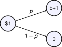
There are two outcomes with returns
\begin{align*} R_1 & = w(b+1) + 1 - w = 1+wb & \mbox{with probability }p\\ R_2 & = 1-w & \mbox{with probability }1-p \end{align*}The expected log return becomes
\begin{align*} E[\ln R] & = p \ln R_1 + (1-p) \ln R_2 \\ & = p\ln(1+ wb) + (1-p)\ln(1-w) \end{align*}Applying Kelly's criterion, we seek a value for $w$ that maximizes $E[\ln R]$. Taking derivatives
\begin{align*} \frac{\partial E[\ln R]}{\partial w} = \frac{pb}{1+w_{opt}b} - \frac{1-p}{1-w_{opt}} & = 0\\ \end{align*}Solving for $w$
$$w_{opt} = \frac{p(b+1)-1}{b}$$The growth rate is then the value of $E[\ln R]$ when $w = w_{opt}$, i.e.,
$$m = p\ln(1+ w_{opt}b) + (1-p)\ln(1-w_{opt})$$You can test how well this works in the following cell. Fix $p$ and $b$, and let the code do a Monte Carlo simulation to show how well Kelly's criterion works.
%matplotlib inline
import numpy as np
import matplotlib.pyplot as plt
from numpy.random import uniform

p = 0.5075
b = 1

# Kelly criterion
w = (p*(b+1)-1)/b

# optimal growth rate
m = p*np.log(1+w*b) + (1-p)*np.log(1-w)

# number of plays to double wealth
K = int(np.log(2)/m)

# monte carlo simulation and plotting
for n in range(0,100):
    W = [1]
    for k in range(0,K):
        if uniform() <= p:
            W.append(W[-1]*(1+w*b))
        else:
            W.append(W[-1]*(1-w))
    plt.semilogy(W,alpha=0.2)
plt.semilogy(np.linspace(0,K), np.exp(m*np.linspace(0,K)),'r',lw=3)
plt.title('Kelly Criterion w = ' + str(round(w,4)))
plt.xlabel('k')
plt.grid()

Example 2. Betting Wheel
%matplotlib inline
import numpy as np
import matplotlib.pyplot as plt


w1 = np.linspace(0,1)
w2 = 0
w3 = 0

p1 = 1/2
p2 = 1/3
p3 = 1/6

R1 = 1 + 2*w1 - w2 - w3
R2 = 1 - w1 + w2 - w3
R3 = 1 - w1 - w2 + 5*w3

m = p1*np.log(R1) + p2*np.log(R2) + p3*np.log(R3)

plt.plot(w1,m)
plt.grid()
/usr/local/lib/python3.6/dist-packages/ipykernel_launcher.py:18: RuntimeWarning: divide by zero encountered in log

def wheel(w,N = 100):
    w1,w2,w3 = w
Example 3. Stock/Bond Portfolio in Continuous Time
%matplotlib inline
import matplotlib.pyplot as plt
import numpy as np
import pandas as pd
import datetime
from pandas_datareader import data, wb
from scipy.stats import norm
import requests
def get_symbol(symbol):
"""
get_symbol(symbol) uses Yahoo to look up a stock trading symbol and
return a description.
"""
url = "http://d.yimg.com/autoc.finance.yahoo.com/autoc?query={}®ion=1&lang=en".format(symbol)
result = requests.get(url).json()
for x in result['ResultSet']['Result']:
if x['symbol'] == symbol:
return x['name']
symbol = '^GSPC'

# end date is today
end = datetime.datetime.today().date()

# start date is three years prior
start = end-datetime.timedelta(1.5*365)

# get stock price data
S = data.DataReader(symbol,"yahoo",start,end)['Adj Close']
rlin = (S - S.shift(1))/S.shift(1)
rlog = np.log(S/S.shift(1))

rlin = rlin.dropna()
rlog = rlog.dropna()

# plot data
plt.figure(figsize=(10,6))
plt.subplot(3,1,1)
S.plot(title=get_symbol(symbol))
plt.ylabel('Adjusted Close')
plt.grid()

plt.subplot(3,1,2)
rlin.plot()
plt.title('Linear Returns (daily)')
plt.grid()
plt.tight_layout()

plt.subplot(3,1,3)
rlog.plot()
plt.title('Log Returns (daily)')
plt.grid()
plt.tight_layout()

print('Linear Returns')
mu,sigma = norm.fit(rlin)
print('   mu = {0:12.8f}  (annualized = {1:.2f}%)'.format(mu,100*252*mu))
print('sigma = {0:12.8f}  (annualized = {1:.2f}%)'.format(sigma,100*np.sqrt(252)*sigma))
print()
print('Log Returns')
nu,sigma = norm.fit(rlog)
print('   nu = {0:12.8f}  (annualized = {1:.2f}%)'.format(nu,100*252*nu))
print('sigma = {0:12.8f}  (annualized = {1:.2f}%)'.format(sigma,100*np.sqrt(252)*sigma))
Linear Returns
   mu =   0.00037731  (annualized = 9.51%)
sigma =   0.00961646  (annualized = 15.27%)

Log Returns
   nu =   0.00033089  (annualized = 8.34%)
sigma =   0.00963609  (annualized = 15.30%)
mu = 252*mu
nu = 252*nu
sigma = np.sqrt(252)*sigma
rf = 0.04
mu = 0.08
sigma = 0.3

w = (mu-rf)/sigma**2
nu_opt = rf + (mu-rf)**2/2/sigma/sigma
sigma_opt = np.sqrt(mu-rf)/sigma

print(w,nu_opt,sigma_opt)
0.4444444444444445 0.04888888888888889 0.6666666666666667
Volatility Pumping
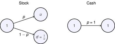
# payoffs for two states
u = 1.059
d = 1/u
p = 0.54

rf = 0.004

K = 100

ElnR = p*np.log(u) + (1-p)*np.log(d)
print("Expected return = {:0.5}".format(ElnR))


Z = np.array([float(random.random() <= p) for _ in range(0,K)])
R = d + (u-d)*Z
S = np.cumprod(np.concatenate(([1],R)))


ElnR = lambda alpha: p*np.log(alpha*u +(1-alpha)*np.exp(rf)) + \
    (1-p)*np.log(alpha*d + (1-alpha)*np.exp(rf))

a = np.linspace(0,1)

plt.plot(a,map(ElnR,a))
Expected return = 0.004586
---------------------------------------------------------------------------
AttributeError                            Traceback (most recent call last)
/usr/local/lib/python3.6/dist-packages/matplotlib/units.py in get_converter(self, x)
    167                 # get_converter
--> 168                 if not np.all(xravel.mask):
    169                     # some elements are not masked

AttributeError: 'numpy.ndarray' object has no attribute 'mask'

During handling of the above exception, another exception occurred:

RuntimeError                              Traceback (most recent call last)
<ipython-input-11-0b509eb701c5> in <module>()
     20 a = np.linspace(0,1)
     21
---> 22 plt.plot(a,map(ElnR,a))

/usr/local/lib/python3.6/dist-packages/matplotlib/pyplot.py in plot(scalex, scaley, data, *args, **kwargs)
   2809     return gca().plot(
   2810         *args, scalex=scalex, scaley=scaley, **({"data": data} if data
-> 2811         is not None else {}), **kwargs)
   2812
   2813

/usr/local/lib/python3.6/dist-packages/matplotlib/__init__.py in inner(ax, data, *args, **kwargs)
   1808                         "the Matplotlib list!)" % (label_namer, func.__name__),
   1809                         RuntimeWarning, stacklevel=2)
-> 1810             return func(ax, *args, **kwargs)
   1811
   1812         inner.__doc__ = _add_data_doc(inner.__doc__,

/usr/local/lib/python3.6/dist-packages/matplotlib/axes/_axes.py in plot(self, scalex, scaley, *args, **kwargs)
   1609         kwargs = cbook.normalize_kwargs(kwargs, mlines.Line2D._alias_map)
   1610
-> 1611         for line in self._get_lines(*args, **kwargs):
   1612             self.add_line(line)
   1613             lines.append(line)

/usr/local/lib/python3.6/dist-packages/matplotlib/axes/_base.py in _grab_next_args(self, *args, **kwargs)
    391                 this += args[0],
    392                 args = args[1:]
--> 393             yield from self._plot_args(this, kwargs)
    394
    395

/usr/local/lib/python3.6/dist-packages/matplotlib/axes/_base.py in _plot_args(self, tup, kwargs)
    368             x, y = index_of(tup[-1])
    369
--> 370         x, y = self._xy_from_xy(x, y)
    371
    372         if self.command == 'plot':

/usr/local/lib/python3.6/dist-packages/matplotlib/axes/_base.py in _xy_from_xy(self, x, y)
    203         if self.axes.xaxis is not None and self.axes.yaxis is not None:
    204             bx = self.axes.xaxis.update_units(x)
--> 205             by = self.axes.yaxis.update_units(y)
    206
    207             if self.command != 'plot':

/usr/local/lib/python3.6/dist-packages/matplotlib/axis.py in update_units(self, data)
   1465         """
   1466
-> 1467         converter = munits.registry.get_converter(data)
   1468         if converter is None:
   1469             return False

/usr/local/lib/python3.6/dist-packages/matplotlib/units.py in get_converter(self, x)
    179                 if (not isinstance(next_item, np.ndarray) or
    180                         next_item.shape != x.shape):
--> 181                     converter = self.get_converter(next_item)
    182                 return converter
    183

/usr/local/lib/python3.6/dist-packages/matplotlib/units.py in get_converter(self, x)
    185         if converter is None:
    186             try:
--> 187                 thisx = safe_first_element(x)
    188             except (TypeError, StopIteration):
    189                 pass

/usr/local/lib/python3.6/dist-packages/matplotlib/cbook/__init__.py in safe_first_element(obj)
   1633         except TypeError:
   1634             pass
-> 1635         raise RuntimeError("matplotlib does not support generators "
   1636                            "as input")
   1637     return next(iter(obj))

RuntimeError: matplotlib does not support generators as input

from scipy.optimize import fminbound
alpha = fminbound(lambda(alpha): -ElnR(alpha),0,1)
print alpha

#plt.plot(alpha, ElnR(alpha),'r.',ms=10)

R = alpha*d + (1-alpha) + alpha*(u-d)*Z
S2 = np.cumprod(np.concatenate(([1],R)))

plt.figure(figsize=(10,4))
plt.plot(range(0,K+1),S,range(0,K+1),S2)
plt.legend(['Stock','Stock + Cash']);
0.5
