Usage example of hrf_estimation
Here we will use real fMRI data to estimate the HRF and activation pattern using the python package hrf_estimation.
For this, we will rely on some publicly available datasets and the hrf_estimation package, which implements the estimation methods described in the publication Data-driven HRF estimation for encoding and decoding models, NeuroImage January 2015
To follow this notebook basic knowledge about fMRI signal processing is assumed.
# import packages we will need
%pylab inline

# nicer plots, but only available in recent matplotlib
try:
    plt.style.use('ggplot')
except:
    pass

import hrf_estimation as he
print('You are running hrf_estimation version %s' % he.__version__)
Populating the interactive namespace from numpy and matplotlib
You are running hrf_estimation version 0.7
Now we will load some sample data. This data is described in the paper “Identifying natural images from human brain activity.,” K. N. Kay et al. Nature 2008, and is publicly available from http://crcns.org. See here for more details and how to obtain the full dataset: http://crcns.org/data-sets/vc/vim-1/about-vim-1 .
The following function will download the data to temporary file in the current directory. It will then load the data and perform a local detrending (Savitzky-Golay filter).
The returned data consist of an array of 500 voxel timecourses, a list of conditions representing the condition ID and a list of onseets representing the time onset of its relative condition. The list of conditions and onsets have the same length. The repetition time (TR) for this dataset is 1 second.
voxels, conditions, onsets = he.data.get_sample_data(0, full_brain=False)
print('Num of timepoints in a single voxel: %s' % voxels.shape[0])
print('Num of voxels: %s' % voxels.shape[1])
print('Num of conditions: %s' % len(conditions))
print('Num of onsets: %s' % len(onsets))
Downloading BOLD signal
Num of timepoints in a single voxel: 3360
Num of voxels: 500
Num of conditions: 700
Num of onsets: 700
This data contains the BOLD time series for 1 session.
In the next step we will detrend the signal using a Savitzky-Golay filter with polynomial of degree three and window length of 121 seconds. The time series for one voxel is plotted after detrending.
### perform detrending: Savitzky-Golay filter
n_voxels = voxels.shape[-1]
voxels = voxels - he.savitzky_golay.savgol_filter(voxels, 91, 3, axis=0)
voxels /= voxels.std(axis=0)
print("Performed detrending of the BOLD timecourse using a Savitzky-Golay filter")

# plot one voxel
plt.figure(figsize=(18, 6))
plt.plot(voxels[:2 * 672, 0], lw=2)
plt.xlabel('Timecourse (in seconds)')
plt.show()
Performed detrending of the BOLD timecourse using a Savitzky-Golay filter

HRF estimation with the Rank-1 GLM (R1GLM) model
We will proceed to estimate the HRF using a R1GLM model.
We will now call the glm function in hrf_estimation. We will use a basis formed by the HRF plus its time and dispersion derivatives. This basis is denoted '3hrf' in this package.
# we construct the matrix of drifts as the matrix of ones that account for
# the intercept term. If you have drifts estimated by e.g. SPM you can add
# them here.
drifts = np.ones((voxels.shape[0], 1))

# we call he.glm with our data and a TR of 1 second. This will return the
# estimated HRF and the
# we also specify the basis function for the HRF estimation
hrfs, betas = he.glm(conditions, onsets, 1., voxels, drifts=drifts, mode='r1glm', basis='3hrf', verbose=1)
.. creating design matrix ..
.. done creating design matrix ..
.. computing initialization ..
.. done initialization ..
.. completed 500 out of 500 ..
The output of he.glm produces estimated HRFs and betas. For the case of 3hrf basis these have been normalized so that the resulting HRF correlates positively with the reference HRF and its maximum value is one.
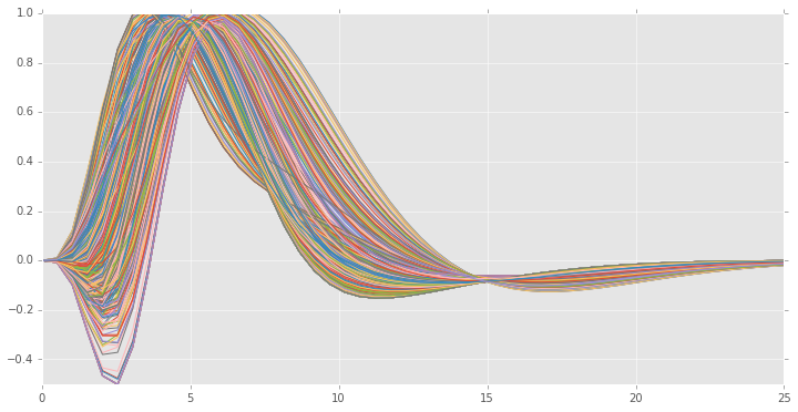
We will now plot the estimated HRFs,
xx = np.linspace(0, 25) # range of values for time
# construct the final HRF by multiplying by its basis
generated_hrfs = hrfs[0] * he.hrf.spmt(xx)[:, None] + hrfs[1] * he.hrf.dspmt(xx)[:, None] + hrfs[2] * he.hrf.ddspmt(xx)[:, None]

plt.figure(figsize=(12, 6))
plt.plot(xx, generated_hrfs)
plt.ylim((-.5, 1.))
plt.show()

Before we have used a 3hrf basis, the basis consisting of the reference HRF plus its time and dispersion derivative. If we only consider the derivative with respect to time we obtain the 2hrf basis. We now fit the same model using a 2hrf basis instead and plot the estimated HRFs
hrfs, betas = he.glm(conditions, onsets, 1., voxels, drifts=drifts, basis='2hrf', verbose=1)
xx = np.linspace(0, 25) # range of values for time
# construct the final HRF by multiplying by its basis
generated_hrfs = hrfs[0] * he.hrf.spmt(xx)[:, None] + hrfs[1] * he.hrf.dspmt(xx)[:, None]

plt.figure(figsize=(12, 6))
plt.plot(xx, generated_hrfs)
plt.ylim((-.5, 1.))
plt.show()
.. creating design matrix ..
.. done creating design matrix ..
.. computing initialization ..
.. done initialization ..
.. completed 500 out of 500 ..

hrfs, betas = he.glm(conditions, onsets, 1., voxels, drifts=drifts, basis='fir', verbose=1)
xx = np.linspace(0, 25) # range of values for time
# construct the final HRF by multiplying by its basis
# generated_hrfs = hrfs[0] * he.hrf.spmt(xx)[:, None] + hrfs[1] * he.hrf.dspmt(xx)[:, None]

plt.figure(figsize=(12, 6))
plt.plot(np.arange(hrfs.shape[0]), hrfs)
plt.ylim((-.5, 1.))
plt.axis('tight')
plt.show()
.. creating design matrix ..
.. done creating design matrix ..
.. computing initialization ..
.. done initialization ..
.. completed 500 out of 500 ..

The measurements here are quite noisy. This is somewhat expected because the FIR basis has many more parameters to estimate than the 3hrf basis and the model is learning noise given the limited time points. This phenomenon is known as overfitting in machine learning. One possible solution is to incorporate more data into the model. We can do this for example by accumulating the data from the different sessions into a big R1-GLM.
In this case we would create a desig matrix in which the diagonal blocks are the design matrices for each of the respective session. This way the HRF will be constrained to be common across the different sessions but we will still have the same number of activation coefficients (beta-map) as if we performed the model for each session individually. The target variable (voxel timecourse) in this model will be simply the concatenation of the timecourse for the considered sessions.
design_all_sessions = []
voxels_all_sessions = []
drifts_all_sessions = []
n_basis = 20
for sess in range(5):
    voxels, conditions, onsets = he.data.get_sample_data(sess, full_brain=False)

    # detrending
    n_voxels = voxels.shape[-1]
    voxels = voxels - he.savitzky_golay.savgol_filter(voxels, 91, 3, axis=0)
    voxels /= voxels.std(axis=0)
    voxels_all_sessions.append(voxels)

    # create design matrix
    design, _ = he.utils.create_design_matrix(conditions, onsets, 1., voxels.shape[0], hrf_length=n_basis, basis='fir')
    design_all_sessions.append(design)
    drifts_all_sessions.append(np.ones((voxels.shape[0], 1)))
Downloading BOLD signal
Downloading BOLD signal
Downloading BOLD signal
Downloading BOLD signal
Downloading BOLD signal
from scipy import sparse
design = sparse.block_diag(design_all_sessions)
drifts = sparse.block_diag(drifts_all_sessions)
out = he.rank_one(design, np.reshape(voxels_all_sessions, (-1, 500)), n_basis, drifts=drifts)
# plot the result
hrfs, beta = out
sign = np.sign(np.dot(hrfs.T, he.hrf.spmt(np.arange(n_basis))))
plt.figure(figsize=(12, 6))
plt.plot(np.arange(hrfs.shape[0]), (sign * hrfs) / np.abs(hrfs).max(0))
#plt.ylim((-.5, 1.))
plt.axis('tight')
plt.show()

This estimation is ness noisy. In the original dataset there are two more sessions (used for validation) that can also be used for the estimation.
GLM with separate designs
It is possible to use other HRF estimating methods besides R1-GLM. For example, the GLM with separate designs can be used by specifying the keyword argument mode='glms'
hrfs, betas = he.glm(conditions, onsets, 1., voxels, drifts=drifts, mode='glms', basis='3hrf', verbose=1)
.. creating design matrix ..
.. done creating design matrix ..
Note however that in this case there is an estimation per event and so the shape of hrfs is (n_basis, n_betas, n_voxels) and thus must be reduced to (n_basis, n_voxels). Here we simply average across conditions.
hrfs_mean = hrfs.mean(1)
generated_hrfs = hrfs_mean[0] * he.hrf.spmt(xx)[:, None] + hrfs_mean[1] * he.hrf.dspmt(xx)[:, None] + \
    hrfs_mean[2] * he.hrf.ddspmt(xx)[:, None]
sign = np.sign(np.dot(generated_hrfs.T, he.hrf.spmt(xx)))
norm = np.abs(generated_hrfs).max(0)
generated_hrfs = generated_hrfs * sign / norm

plt.figure(figsize=(12, 6))
plt.plot(generated_hrfs)
plt.ylim((-1., 1.))
plt.show()
