Model selection and evaluation
Model selection and evaluation is one of the most important things in data ming and machine learning. These are the following topics you must understand:
- Bias vs Variance Tradeoff
- Cross Validation and combatting over and under fitting
What do do next? (advanced topics)
- Model Evaluation using learning curves
- Grid Search: Searching for estimator parameters
The scikit-learn documentation is great: http://scikit-learn.org/stable/model_selection.html
http://scikit-learn.org/stable/tutorial/statistical_inference/index.html#stat-learn-tut-index
Bias vs Variance Tradeoff

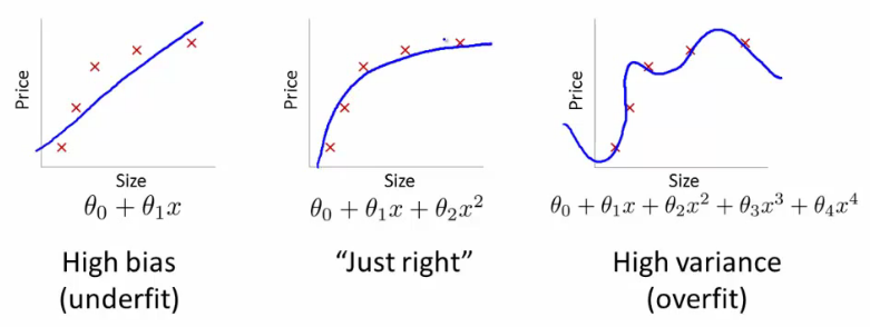
There are three types of error in a model:
a. Bias: difference between the expected (or average) prediction of our model and the correct value which we are trying to predict.
High bias can cause an algorithm to miss the relevant relations between features and target outputs (underfitting)
b. Variance: error due to variance is taken as the variability of a model prediction for a given data point
High variance can cause overfitting: modeling the random noise in the training data, rather than the intended outputs.
c. Irreducible error
Real world data will almost always have irreducible errors. These errors are what cause underfitting and overfitting and are very difficult to determine (since you never have all of the data with most machine learning problems)
https://en.wikipedia.org/wiki/Bias%E2%80%93variance_tradeoff
http://scott.fortmann-roe.com/docs/BiasVariance.html
Over and under fitting
print(__doc__)

import numpy as np
import matplotlib.pyplot as plt
from sklearn.pipeline import Pipeline
from sklearn.preprocessing import PolynomialFeatures
from sklearn.linear_model import LinearRegression
from sklearn import cross_validation
%matplotlib inline
np.random.seed(0)

n_samples = 30
degrees = [1, 4, 15]

true_fun = lambda X: np.cos(1.5 * np.pi * X)
X = np.sort(np.random.rand(n_samples))
y = true_fun(X) + np.random.randn(n_samples) * 0.1

plt.figure(figsize=(14, 5))
for i in range(len(degrees)):
    ax = plt.subplot(1, len(degrees), i + 1)
    plt.setp(ax, xticks=(), yticks=())

    polynomial_features = PolynomialFeatures(degree=degrees[i],
                                             include_bias=False)
    linear_regression = LinearRegression()
    pipeline = Pipeline([("polynomial_features", polynomial_features),
                         ("linear_regression", linear_regression)])
    pipeline.fit(X[:, np.newaxis], y)

    # Evaluate the models using crossvalidation
    scores = cross_validation.cross_val_score(pipeline,
        X[:, np.newaxis], y, scoring="mean_squared_error", cv=10)

    X_test = np.linspace(0, 1, 100)
    plt.plot(X_test, pipeline.predict(X_test[:, np.newaxis]), label="Model")
    plt.plot(X_test, true_fun(X_test), label="True function")
    plt.scatter(X, y, label="Samples")
    plt.xlabel("x")
    plt.ylabel("y")
    plt.xlim((0, 1))
    plt.ylim((-2, 2))
    plt.legend(loc="best")
    plt.title("Degree {}\nMSE = {:.2e}(+/- {:.2e})".format(
        degrees[i], -scores.mean(), scores.std()))
plt.show()
Automatically created module for IPython interactive environment

Cross Validation
While the holdout method is the simpliest, you should be using K folds cross validation. The general rule of thumb is to use 10 folds.
Another important part of cross validation is the metric you are using to score the algorithm:
Model evaluation: quantifying the quality of predictions
https://en.wikipedia.org/wiki/Confusion_matrix
Deciding the correct metric is the first and very important set!
print(__doc__)

import numpy as np
from scipy import interp
import matplotlib.pyplot as plt

from sklearn import svm, datasets
from sklearn.metrics import roc_curve, auc
from sklearn.cross_validation import StratifiedKFold

###############################################################################
# Data IO and generation

# import some data to play with
iris = datasets.load_iris()
X = iris.data
y = iris.target
X, y = X[y != 2], y[y != 2]
n_samples, n_features = X.shape

# Add noisy features
random_state = np.random.RandomState(0)
X = np.c_[X, random_state.randn(n_samples, 200 * n_features)]

###############################################################################
# Classification and ROC analysis

# Run classifier with cross-validation and plot ROC curves
cv = StratifiedKFold(y, n_folds=6)
classifier = svm.SVC(kernel='linear', probability=True,
                     random_state=random_state)

mean_tpr = 0.0
mean_fpr = np.linspace(0, 1, 100)
all_tpr = []

for i, (train, test) in enumerate(cv):
    probas_ = classifier.fit(X[train], y[train]).predict_proba(X[test])
    # Compute ROC curve and area the curve
    fpr, tpr, thresholds = roc_curve(y[test], probas_[:, 1])
    mean_tpr += interp(mean_fpr, fpr, tpr)
    mean_tpr[0] = 0.0
    roc_auc = auc(fpr, tpr)
    plt.plot(fpr, tpr, lw=1, label='ROC fold %d (area = %0.2f)' % (i, roc_auc))

plt.plot([0, 1], [0, 1], '--', color=(0.6, 0.6, 0.6), label='Luck')

mean_tpr /= len(cv)
mean_tpr[-1] = 1.0
mean_auc = auc(mean_fpr, mean_tpr)
plt.plot(mean_fpr, mean_tpr, 'k--',
         label='Mean ROC (area = %0.2f)' % mean_auc, lw=2)

plt.xlim([-0.05, 1.05])
plt.ylim([-0.05, 1.05])
plt.xlabel('False Positive Rate')
plt.ylabel('True Positive Rate')
plt.title('Receiver operating characteristic example')
plt.legend(loc="lower right")
plt.show()
Automatically created module for IPython interactive environment

3. Determining Parameters
After selecting a model you can tune the parameters.
print(__doc__)

import matplotlib.pyplot as plt
import numpy as np
from sklearn.datasets import load_digits
from sklearn.svm import SVC
from sklearn.learning_curve import validation_curve

digits = load_digits()
X, y = digits.data, digits.target

param_range = np.logspace(-6, -1, 5)
train_scores, test_scores = validation_curve(
    SVC(), X, y, param_name="gamma", param_range=param_range,
    cv=10, scoring="accuracy", n_jobs=1)
train_scores_mean = np.mean(train_scores, axis=1)
train_scores_std = np.std(train_scores, axis=1)
test_scores_mean = np.mean(test_scores, axis=1)
test_scores_std = np.std(test_scores, axis=1)

plt.title("Validation Curve with SVM")
plt.xlabel("$\gamma$")
plt.ylabel("Score")
plt.ylim(0.0, 1.1)
plt.semilogx(param_range, train_scores_mean, label="Training score", color="r")
plt.fill_between(param_range, train_scores_mean - train_scores_std,
                 train_scores_mean + train_scores_std, alpha=0.2, color="r")
plt.semilogx(param_range, test_scores_mean, label="Cross-validation score",
             color="g")
plt.fill_between(param_range, test_scores_mean - test_scores_std,
                 test_scores_mean + test_scores_std, alpha=0.2, color="g")
plt.legend(loc="best")
plt.show()
Automatically created module for IPython interactive environment

from __future__ import print_function

from pprint import pprint
from time import time
import logging

from sklearn.datasets import fetch_20newsgroups
from sklearn.feature_extraction.text import CountVectorizer
from sklearn.feature_extraction.text import TfidfTransformer
from sklearn.linear_model import SGDClassifier
from sklearn.grid_search import GridSearchCV
from sklearn.pipeline import Pipeline

print(__doc__)

# Display progress logs on stdout
logging.basicConfig(level=logging.INFO,
                    format='%(asctime)s %(levelname)s %(message)s')


###############################################################################
# Load some categories from the training set
categories = [
    'alt.atheism',
    'talk.religion.misc',
]
# Uncomment the following to do the analysis on all the categories
#categories = None

print("Loading 20 newsgroups dataset for categories:")
print(categories)

data = fetch_20newsgroups(subset='train', categories=categories)
print("%d documents" % len(data.filenames))
print("%d categories" % len(data.target_names))
print()

###############################################################################
# define a pipeline combining a text feature extractor with a simple
# classifier
pipeline = Pipeline([
    ('vect', CountVectorizer()),
    ('tfidf', TfidfTransformer()),
    ('clf', SGDClassifier()),
])

# uncommenting more parameters will give better exploring power but will
# increase processing time in a combinatorial way
parameters = {
    'vect__max_df': (0.5, 0.75, 1.0),
    #'vect__max_features': (None, 5000, 10000, 50000),
    'vect__ngram_range': ((1, 1), (1, 2)),  # unigrams or bigrams
    #'tfidf__use_idf': (True, False),
    #'tfidf__norm': ('l1', 'l2'),
    'clf__alpha': (0.00001, 0.000001),
    'clf__penalty': ('l2', 'elasticnet'),
    #'clf__n_iter': (10, 50, 80),
}

if __name__ == "__main__":
    # multiprocessing requires the fork to happen in a __main__ protected
    # block

    # find the best parameters for both the feature extraction and the
    # classifier
    grid_search = GridSearchCV(pipeline, parameters, n_jobs=-1, verbose=1)

    print("Performing grid search...")
    print("pipeline:", [name for name, _ in pipeline.steps])
    print("parameters:")
    pprint(parameters)
    t0 = time()
    grid_search.fit(data.data, data.target)
    print("done in %0.3fs" % (time() - t0))
    print()

    print("Best score: %0.3f" % grid_search.best_score_)
    print("Best parameters set:")
    best_parameters = grid_search.best_estimator_.get_params()
    for param_name in sorted(parameters.keys()):
        print("\t%s: %r" % (param_name, best_parameters[param_name]))
Automatically created module for IPython interactive environment
Loading 20 newsgroups dataset for categories:
['alt.atheism', 'talk.religion.misc']
857 documents
2 categories

Performing grid search...
pipeline: ['vect', 'tfidf', 'clf']
parameters:
{'clf__alpha': (1e-05, 1e-06),
 'clf__penalty': ('l2', 'elasticnet'),
 'vect__max_df': (0.5, 0.75, 1.0),
 'vect__ngram_range': ((1, 1), (1, 2))}
Fitting 3 folds for each of 24 candidates, totalling 72 fits
[Parallel(n_jobs=-1)]: Done  42 tasks      | elapsed:   17.4s
[Parallel(n_jobs=-1)]: Done  72 out of  72 | elapsed:   30.2s finished
done in 30.773s

Best score: 0.938
Best parameters set:
	clf__alpha: 1e-05
	clf__penalty: 'l2'
	vect__max_df: 0.75
	vect__ngram_range: (1, 1)
print(__doc__)

import numpy as np

from time import time
from operator import itemgetter
from scipy.stats import randint as sp_randint

from sklearn.grid_search import GridSearchCV, RandomizedSearchCV
from sklearn.datasets import load_digits
from sklearn.ensemble import RandomForestClassifier

# get some data
digits = load_digits()
X, y = digits.data, digits.target

# build a classifier
clf = RandomForestClassifier(n_estimators=20)


# Utility function to report best scores
def report(grid_scores, n_top=3):
    top_scores = sorted(grid_scores, key=itemgetter(1), reverse=True)[:n_top]
    for i, score in enumerate(top_scores):
        print("Model with rank: {0}".format(i + 1))
        print("Mean validation score: {0:.3f} (std: {1:.3f})".format(
              score.mean_validation_score,
              np.std(score.cv_validation_scores)))
        print("Parameters: {0}".format(score.parameters))
        print("")


# specify parameters and distributions to sample from
param_dist = {"max_depth": [3, None],
              "max_features": sp_randint(1, 11),
              "min_samples_split": sp_randint(1, 11),
              "min_samples_leaf": sp_randint(1, 11),
              "bootstrap": [True, False],
              "criterion": ["gini", "entropy"]}

# run randomized search
n_iter_search = 20
random_search = RandomizedSearchCV(clf, param_distributions=param_dist,
                                   n_iter=n_iter_search)

start = time()
random_search.fit(X, y)
print("RandomizedSearchCV took %.2f seconds for %d candidates"
      " parameter settings." % ((time() - start), n_iter_search))
report(random_search.grid_scores_)

# use a full grid over all parameters
param_grid = {"max_depth": [3, None],
              "max_features": [1, 3, 10],
              "min_samples_split": [1, 3, 10],
              "min_samples_leaf": [1, 3, 10],
              "bootstrap": [True, False],
              "criterion": ["gini", "entropy"]}

# run grid search
grid_search = GridSearchCV(clf, param_grid=param_grid)
start = time()
grid_search.fit(X, y)

print("GridSearchCV took %.2f seconds for %d candidate parameter settings."
      % (time() - start, len(grid_search.grid_scores_)))
report(grid_search.grid_scores_)
Automatically created module for IPython interactive environment
RandomizedSearchCV took 4.76 seconds for 20 candidates parameter settings.
Model with rank: 1
Mean validation score: 0.926 (std: 0.014)
Parameters: {'bootstrap': False, 'min_samples_leaf': 3, 'min_samples_split': 6, 'criterion': 'gini', 'max_features': 8, 'max_depth': None}

Model with rank: 2
Mean validation score: 0.919 (std: 0.017)
Parameters: {'bootstrap': False, 'min_samples_leaf': 4, 'min_samples_split': 3, 'criterion': 'entropy', 'max_features': 10, 'max_depth': None}

Model with rank: 3
Mean validation score: 0.919 (std: 0.011)
Parameters: {'bootstrap': True, 'min_samples_leaf': 3, 'min_samples_split': 4, 'criterion': 'gini', 'max_features': 3, 'max_depth': None}

GridSearchCV took 46.52 seconds for 216 candidate parameter settings.
Model with rank: 1
Mean validation score: 0.932 (std: 0.004)
Parameters: {'bootstrap': False, 'min_samples_leaf': 1, 'min_samples_split': 3, 'criterion': 'gini', 'max_features': 3, 'max_depth': None}

Model with rank: 2
Mean validation score: 0.931 (std: 0.017)
Parameters: {'bootstrap': False, 'min_samples_leaf': 1, 'min_samples_split': 3, 'criterion': 'entropy', 'max_features': 10, 'max_depth': None}

Model with rank: 3
Mean validation score: 0.928 (std: 0.009)
Parameters: {'bootstrap': True, 'min_samples_leaf': 1, 'min_samples_split': 3, 'criterion': 'entropy', 'max_features': 10, 'max_depth': None}
print(__doc__)

import numpy as np
import matplotlib.pyplot as plt
from sklearn import cross_validation
from sklearn.naive_bayes import GaussianNB
from sklearn.svm import SVC
from sklearn.datasets import load_digits
from sklearn.learning_curve import learning_curve


def plot_learning_curve(estimator, title, X, y, ylim=None, cv=None,
                        n_jobs=1, train_sizes=np.linspace(.1, 1.0, 5)):
    """
    Generate a simple plot of the test and traning learning curve.

    Parameters
    ----------
    estimator : object type that implements the "fit" and "predict" methods
        An object of that type which is cloned for each validation.

    title : string
        Title for the chart.

    X : array-like, shape (n_samples, n_features)
        Training vector, where n_samples is the number of samples and
        n_features is the number of features.

    y : array-like, shape (n_samples) or (n_samples, n_features), optional
        Target relative to X for classification or regression;
        None for unsupervised learning.

    ylim : tuple, shape (ymin, ymax), optional
        Defines minimum and maximum yvalues plotted.

    cv : integer, cross-validation generator, optional
        If an integer is passed, it is the number of folds (defaults to 3).
        Specific cross-validation objects can be passed, see
        sklearn.cross_validation module for the list of possible objects

    n_jobs : integer, optional
        Number of jobs to run in parallel (default 1).
    """
    plt.figure()
    plt.title(title)
    if ylim is not None:
        plt.ylim(*ylim)
    plt.xlabel("Training examples")
    plt.ylabel("Score")
    train_sizes, train_scores, test_scores = learning_curve(
        estimator, X, y, cv=cv, n_jobs=n_jobs, train_sizes=train_sizes)
    train_scores_mean = np.mean(train_scores, axis=1)
    train_scores_std = np.std(train_scores, axis=1)
    test_scores_mean = np.mean(test_scores, axis=1)
    test_scores_std = np.std(test_scores, axis=1)
    plt.grid()

    plt.fill_between(train_sizes, train_scores_mean - train_scores_std,
                     train_scores_mean + train_scores_std, alpha=0.1,
                     color="r")
    plt.fill_between(train_sizes, test_scores_mean - test_scores_std,
                     test_scores_mean + test_scores_std, alpha=0.1, color="g")
    plt.plot(train_sizes, train_scores_mean, 'o-', color="r",
             label="Training score")
    plt.plot(train_sizes, test_scores_mean, 'o-', color="g",
             label="Cross-validation score")

    plt.legend(loc="best")
    return plt


digits = load_digits()
X, y = digits.data, digits.target


title = "Learning Curves (Naive Bayes)"
# Cross validation with 100 iterations to get smoother mean test and train
# score curves, each time with 20% data randomly selected as a validation set.
cv = cross_validation.ShuffleSplit(digits.data.shape[0], n_iter=100,
                                   test_size=0.2, random_state=0)

estimator = GaussianNB()
plot_learning_curve(estimator, title, X, y, ylim=(0.7, 1.01), cv=cv, n_jobs=4)

title = "Learning Curves (SVM, RBF kernel, $\gamma=0.001$)"
# SVC is more expensive so we do a lower number of CV iterations:
cv = cross_validation.ShuffleSplit(digits.data.shape[0], n_iter=10,
                                   test_size=0.2, random_state=0)
estimator = SVC(gamma=0.001)
plot_learning_curve(estimator, title, X, y, (0.7, 1.01), cv=cv, n_jobs=4)

plt.show()
Automatically created module for IPython interactive environment

