Lecture 9: Meta-Learning
Ensembles: $n$ Heads are Better than One
In a previous assignment, we had you analyze the Titanic dataset on Kaggle. You may have noticed that Kaggle competitions boast thousands of participants, many of whom are professional data scientists. Out of all of these participants, many of whom are using the models we learned in class, how does a winner emerge?
Is it in the way that they clean and process their data? Perhaps, but cleaning data can only go so far to improve predictive power. Ultimately, success is in the selection and optimization of models. We've seen some techniques for this in lecture 7 (like PCA), but many Kagglers take things even further. Let's see what the first-place Kaggle user, Gilberto Titericz Jr, used for the Otto Product Classification Challenge [1]:

Titericz's solution contained several layers, each containing a blend of learning models. We'll now learn why this is the case.
Review: Bias-Variance Tradeoff
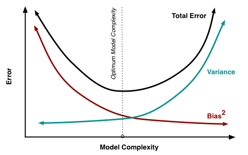
Why do several models perform better than a single model? Recall our discussion of goodness of fit - a model is often prone to either underfitting or overfitting. Another way to look at this dichotomy is as a tradeoff between bias and variance.
Bias is another word for "systematic error." This is error that can occur because a model is underdeveloped or undertrained - in other words, it is inadequate for the task it is attempting to perform. Imagine, for example, using a linear model to fit a relationship that is clearly quadratic or cubic. Some of the relationship would be captured, and occasionally the model would get things right. But as a whole, this linear model would have all-around poor performance. We call this underfitting.
Variance can be thought of as "random error." This, in contrast with bias, occurs because a model is overly sophisticated or complex for the task at hand. The model would perform very well on the training data, but as soon as the data is varied slightly - as soon as we move to a testing set, for example - this model would perform poorly. An example of this is fitting a degree-9 polynomial to a relationship that is quadratic or cubic. As we saw last lecture, this is an example of overfitting.
The bias-variance tradeoff states that for a single machine learning model, bias and variance cannot be reduced simultaneously: [2]
We have already seen methods for reducing variance (regularization), but there are other recently-developed methods for reducing both bias and variance. These methods, also called ensemble methods, bypass the bias-variance tradeoff by employing a mix of many models. The usage of many models increases predictive power, and the blending of these models together into a single output reduces variance.
We'll examine a few types of ensembles: boosting, bagging, and stacking.
Boosting
The Idea
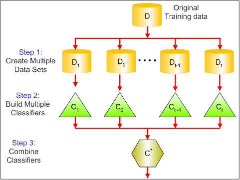
Boosting is a sequential ensemble method: we start from an ineffective machine learning model and gradually "boost" it up, increasing its predictive abilities in each time step. The method by which we improve this model is underspecified, and each specific boosting implementation performs it differently.
Generally, the improvement method is as follows: take the parts of the data where the model has done poorly and retrain a new version of the model on this "failed" data. We then combine this new version with the old version, hoping that this combination performs better than the old version alone [3].
Below is a diagram of a boosted model. Note how each model is trained on a different set of data based on the strengths of the others [4]:

When boosting, our starting point (the very first model used) is often called a weak learner. The power of this starting point doesn't matter much, since the output of a boosting procedure (if done correctly) should be stronger than any individual model.
Example: AdaBoost
AdaBoost is a widely used boosting framework which uses the procedure described above on decision trees. Each iteration of the decision tree created by AdaBoost weights incorrectly classified data more heavily than the previous tree. We continue the process a given number of times until we're satisfied, and then return the weighted sum of all of the decision trees [5].
# Use adaboost
library(adabag)
boost_fit <- boosting(formula, data, boos = TRUE, mfinal = 100, coeflearn = 'Breiman', control,...)
Error in library(adabag): there is no package called 'adabag'
Traceback:

1. library(adabag)
2. stop(txt, domain = NA)
Example: XGBoost
XGBoost uses another paradigm: the idea of gradient descent. We take some cost function that tells us how poorly the ensemble is performing. We then take the gradient of this cost function. This is the direction of maximum decrease; this is the direction we'd like to go in since we want to minimize the cost function. We then adjust the next tree such that the cost function moves in the direction of this gradient [6].
# Use xgboost
library(xgboost)
xgboost_fit <- xgboost(data = train$data, label = train$label, max.depth = 2, eta = 1, nthread = 2, nround = 2, objective = "binary:logistic")
Bagging
The Idea
Bagging, also known as Bootstrap aggregating, is a parallel ensemble method. Before talking more about Bootstrap Aggregating ensemble, we might want to understand what Bootstrap is; bootstrap is choosing a random sample from the dataset with replacement (in our context, it will be getting a random subset() from the original data.frame with replacement). Therefore, bootstrap agggregating is to choose multiple bootstrap samples, train them separately and independently (thus, a parallel method as mentioned above), and combine (or aggregate) each trained model's result as a whole.
More formal definition is: Bagging is a parallel ensemble method: we run a host of models in parallel on a dataset, averaging or aggregating their results in some way. Each model runs on a randomly selected subset of the data, and all models are trained independently of the others (contrast this with boosting).
The primary goal of bagging is to reduce variance. Bagging does not necessarily improve predictive power; instead it is mainly used to prevent overfitting [7]. Below is a diagram of a typical bagging process [8]:
Example: Random Forest
An example of bagging applied to decision trees is the popular random forest model. Random forests create decision trees which are randomly trained on the data. The final output of a given test point is the average of the outputs of all of the randomly trained trees on that point.
cancer <- read.csv("breast_cancer.csv")

set.seed(2017)
ind <- sample(nrow(cancer),0.8*nrow(cancer))
train <- cancer[ind,]
test <- cancer[-ind,]

library(randomForest)
rf <- randomForest(diagnosis ~ .,
                   data = train[,2:10],
                   ntree = 20)
pred <- predict(rf, newdata = test[,-c(length(test))])
cm <- table(test$diagnosis, pred)
cm
   pred
     B  M
  B 84  1
  M  3 26
Stacking
The Idea
Stacking is perhaps the epitome of meta-learning: stacked models perform machine learning on other models. We take various models (often with different features or different learning algorithms) and train them on random subsets (folds) of our data. We then perform another machine learning model - for instance, linear or logistic regression - on the outputs of these models to obtain a final value [9]. Using a regression model gives us a weighted sum of all of the models - much like what we see in the Kaggle winner's diagram.
Here is a diagram of stacking [10]:
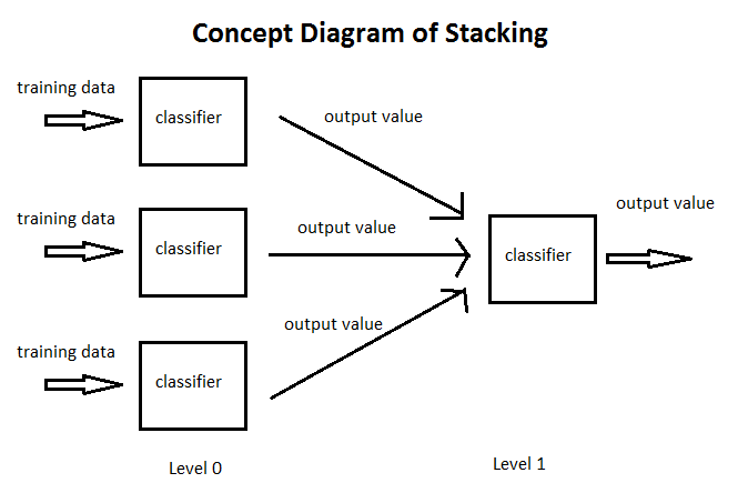
It is important to train each model on a random subset of the data. Otherwise, the stacked model will simply lean towards the most accurate model in the set of models and ignore others. Random subsetting is important for achieving the right "blend" of model weights.
Terms to Review
- Ensemble
- Bias
- Variance
- Boosting
- Weak learner
- AdaBoost
- XGBoost
- Gradient descent
- Bagging (bootstrap aggregating)
- Random forest
- Stacking
Sources
[1] https://kaggle2.blob.core.windows.net/forum-message-attachments/79598/2514/FINAL_ARCHITECTURE.png
[2] http://scott.fortmann-roe.com/docs/docs/BiasVariance/biasvariance.png
[3] https://stats.stackexchange.com/questions/256/how-does-boosting-work
[4] https://codesachin.files.wordpress.com/2016/03/boosting_new_fit5.png?w=491&h=275
[5] https://www.quora.com/What-is-AdaBoost/answer/Janu-Verma-2
[6] http://xgboost.readthedocs.io/en/latest/model.html
[7] https://stats.stackexchange.com/questions/18891/bagging-boosting-and-stacking-in-machine-learning
[8] https://www.analyticsvidhya.com/wp-content/uploads/2015/09/bagging.png
[9] https://mlwave.com/kaggle-ensembling-guide/
[10] http://www.chioka.in/wp-content/uploads/2013/09/stacking.png