Lecture 8: Model Selection and Optimization
We've covered a lot of ground in the past seven lectures. We've become acquainted with:
- The quirks of the R programming language
- Visualization best practices and the
ggplot2package - Linear regression, logistic regression, and decision trees
- A slew of classifiers ($k$-nearest neighbor, naive Bayes, and support vector machines)
- Clustering and unsupervised learning
We'll spend the last four lectures covering a few advanced topics that we think data scientists should know. Today our focus is on a crucial component of data science: how to make models more powerful and efficient.
Leveling Up
So far we've learned plenty of facts about models and problems in data science. By now, you've built up an impressive toolkit of ideas and concepts. But one thing we haven't yet covered in detail is the judicious application of these tools in the right place at the right time. We hope that this lecture will help you "level up" as a data scientist and understand the deeper unifying principles behind the algorithms we're learning.
Bias-Variance Tradeoff
An important thing to recognize when it comes to machine learning is that there is rarely a single perfect model. The real world is rife with noise and imperfection; in practically all cases, we can't build a mathematical model that perfectly encapsulates what is going on. Instead, we make tradeoffs between different types of error depending on our situation.
The error for a model can be broken down into three parts:
$$ Error = (Bias)^2 + Variance + \epsilon $$Let's see what each of these means.
Bias is also known as "systematic error." It is a consistent error that appears because the model is too simple or undertrained or is insufficient to accurately fit the data. An example of this could be attempting to fit a simple linear regression model with a single feature to a problem with 10 significant features.
Variance is also known as "random error." It is an error that appears because the model is too rigid or overtrained and cannot account for deviations or fluctuations in the data. An example of this could be attempting to fit a quadratic regression model to a dataset whose true underlying relationship is linear.
Irreducible error $\epsilon$ is an inevitable part of any model due to the inherent differences between reality and mathematical modeling. It cannot be eliminated.
The bias-variance tradeoff, as it's commonly known, is present because eliminating bias creates the risk of increased variance and vice versa. It's easy to see why: complexify a simplistic model and you run the risk of being overly complex. Simplify a complex model and you run the risk of being overly simplistic. The best models find the balance between the two.
A graph of bias vs. variance is below [4]:
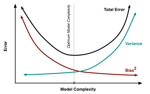
An example of a bias-variance graph is shown above. A good model in this situation would be one where both bias and variance are minimized (i.e. a local minimum in the total error curve). In practice, you could try plotting a chart of the total test error and finding empirically where it is lowest. If the test set is unavailable, you can use cross-validation (which will be discussed later in this lecture).
Overfitting and Underfitting
One common misconception is that if we build a model that has an error close to 0 in the training set, this will necessarily lead to a near-perfect model on the test set. As we're about to see, this is untrue.
We can extend the concepts of bias and variance to define overfitting and underfitting:
- Overfitting is when a model has high variance and low bias.
- Underfitting is when a model has high bias and low variance.
Note that overfitting and underfitting are not necessarily synonyms for variance and bias. Over/underfit are adjectives used to describe a model; bias and variance are components of a model's error.
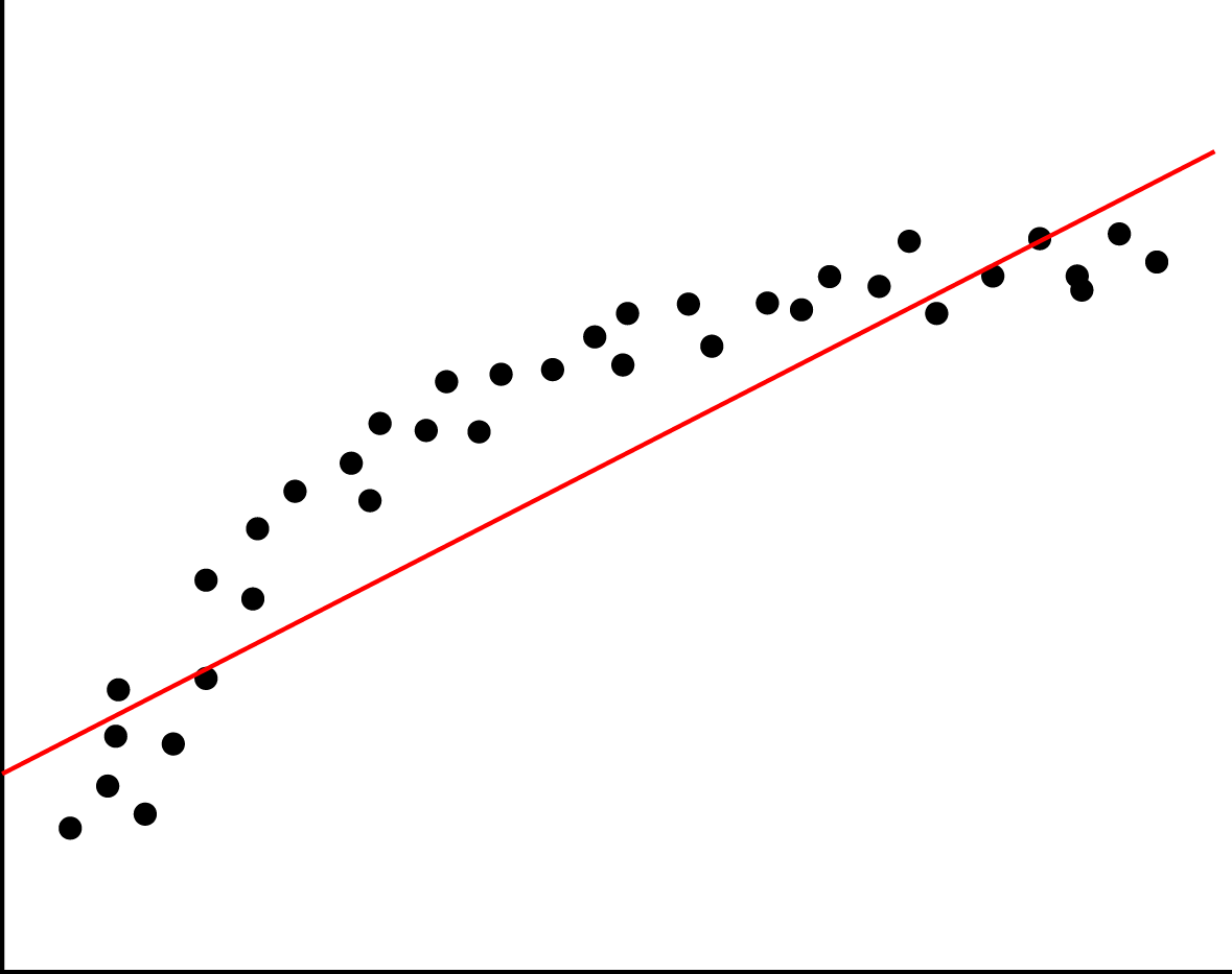
Here is a model that is underfitted [5]:
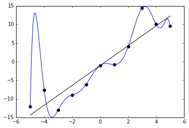
Here is a model that is overfitted [6]:
Feature Selection
As we know, data comes in the form of matrices: observations are rows and variables are columns. We refer to these variables as features.
One way to avoid overfitting is to be frugal (and, yes, parsimonious) with which features we include in the model. Including unnecessary features can also be a waste of computing resources and development time. This part of data science is well documented and studied, and is called feature selection. We'll focus on two important feature selection algorithms today.
If you've taken a discrete math class (CS 2800 at Cornell), you'll know that any set of $p$ elements contains $2^p$ subsets of elements. This exponential relationship between set size and number of subsets spells bad news for our feature selection problem: even for a small number of features like 20, we now have 1,048,576 possible models to test. Any brute-force solution is inefficient.
Two popular greedy algorithms avoid these problems of inefficiency with near-optimal outcomes. They belong to a class of algorithms called subset selection methods. Forward subset selection is as follows:
- Start with no features.
- Add a potential feature and run the model on test data. Keep track of the error.
- Keep the potential feature that decreases the test data the most. Repeat step 2.
- Continue until improvements are negligible.
Backward subset selection is as follows:
- Start with all features.
- Remove the feature with the highest $p$-value (i.e. is least significant).
- Check the model again and repeat step 2. (Note: it's important to rebuild the entire model before checking $p$-values.)
- Continue until all features have a $p$-value below a certain threshold.
Both of these are "hill-climbing" algorithms: they are good at finding locally optimal solutions due to continuous improvement, but the globally optimal solution is not guaranteed. In most cases, they work pretty well.
Validation / Cross Validation
Since training and testing error are so different, it's crucial to always have a testing set on hand to verify how the model will perform "in the wild." Sometimes, though, we can't use the testing set: it's unavailable, too large or small, or it doesn't exist yet. In this case, we have to be parsimonious with our data and use cross validation to approximate our testing error using our training set.
The simplest type of cross validation is the validation set method. This is when part of the training set is allocated as the "validation set", or a pseudo-training set. The model is trained on the non-validation portion and is tested on the validation portion.
Here is an example of the validation set breakdown [7]:

There are three other notable cross validation methods:
Leave-$p$-out cross validation - For each data point, leave out $p$ points and train the model on the rest of the points. Then compute the test error on the $p$ points you've left out.
The overall cross validated error is the average of all of these error values.
$k$-fold cross validation - Create $k$ partitions (folds) of the data. For each fold, treat the other $k-1$ folds as the training data and the remaining fold as the testing data. Compute the test error.
The overall cross validated error is the average of all of these error values.
Regularization
To be parsimonious, we should take steps to reduce the complexity of the models we're dealing with. The class of techniques used for reducing model complexity is called regularization.
Take linear regression for example. We've seen that we can approximate how well a linear regression model is doing by using the training loss, defined as follows:
$$ SSE = \sum_{i = 1}^n (y_i - \hat{y_i})^2 $$However, this error tends to grow smaller as we add more features - this apparent gain in accuracy is misleading, since we're making the model more complex. As a result, we should add a term to this that grows larger with the number of features we're using. This naturally penalizes models that are unnecessarily complex.
We'll cover two techniques of regularization for regression. One is called ridge regression. This is the same as standard linear regression, except we modify the training loss equation to the following:
$$ SSE = \sum_{i = 1}^n (y_i - \hat{y_i})^2 + \lambda \sum_{j=1}^p \beta^2_j $$The coefficient of the extra term, $\lambda$, is called the penalty threshold constant. Make this larger/smaller to increase/decrease the impact of the regularization term (also called regularization loss). The sum of squared $\beta$ values is called the $L_2$ regularization penalty.
Ridge regression is useful for predictor variables that are correlated and not sparse, and when the predictors have small individual effects. The regularization term limits the magnitudes of the coefficients but does not completely eliminate them. Contrast this with lasso regression below.
A related regularization technique is called lasso regression. The training loss in this case is:
$$ SSE = \sum_{i = 1}^n (y_i - \hat{y_i})^2 + \lambda \sum_{j=1}^p |\beta_j| $$Note that an absolute value is used in the equation for lasso regression. We call this the $L_1$ regularization penalty. This behaves differently from ridge regression since it can drive coefficients to 0 when $\lambda$ is large enough. In this sense, lasso regression is a form of feature selection. Note that lasso regression performs better on sparse, uncorrelated variables (contrast this with ridge regression).
Terms to Review
- Parsimony
- Occam's Razor
- Bias
- Variance
- Irreducible error
- Overfitting
- Underfitting
- Feature
- Feature selection
- Forward subset selection
- Backward subset selection
- Validation set
- Leave-one-out/Leave-$p$-out cross validation
- $k$-fold cross validation
- Regularization
- Ridge regression
- Lasso regression
Sources
[1] https://archosaurmusings.wordpress.com/2008/06/15/the-principle-of-parsimony-in-science/
[2] https://www.google.com/search?q=parsimonious
[3] http://math.ucr.edu/home/baez/physics/General/occam.html
[4] http://scott.fortmann-roe.com/docs/docs/BiasVariance/biasvariance.png
[5] https://xyclade.github.io/MachineLearning/Images/Under-fitting.png
[6] https://upload.wikimedia.org/wikipedia/commons/6/68/Overfitted_Data.png
[7] https://www.intechopen.com/source/html/39037/media/image3.jpeg