from IPython.core.display import HTML
css_file = 'css/ngcmstyle.css'
HTML(open(css_file, "r").read())
%matplotlib inline

#rcParams['figure.figsize'] = (10,3) #wide graphs by default
import scipy
import numpy as np
import time
from sympy import symbols,diff,pprint,sqrt,exp,sin,cos,log,Matrix,Function,solve


from mpl_toolkits.mplot3d import Axes3D
from IPython.display import clear_output,display,Math
import matplotlib.pylab as plt
Partial Differentiation
Definition
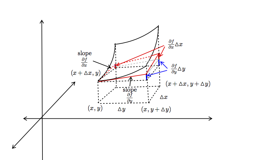
Suppose that $(x_0, y_0)$ is in the domain of $z = f (x, y)$ 1. the partial derivative with respect to $x$ at $(x_0, y_0)$ is the limit
$$ \mathbf{\frac{\partial f}{\partial x} (x_0, y_0) = \lim_{h \rightarrow 0} \frac{f (x_0 + h, y_0) - f (x_0, y_0)}{h} }$$Geometrically, the value of this limit is the slope of the tangent line of $z = f (x, y)$ in the plane $y = y_0$. And this quantity is the rate of change of $f (x, y)$ at $(x_0, y_0)$ along the $x$-direction.
2. the partial derivative with respect to $y$ at $(x_0, y_0)$ is the limit
$$\mathbf{ \frac{\partial f}{\partial y} (x_0, y_0) = \lim_{k \rightarrow 0} \frac{f (x_0, y_0 + k) - f (x_0, y_0)}{k} }$$Geometrically, the value of this limit is the slope of the tangent line of $z = f (x, y)$ in the plane $x = x_0$. And this quantity is the rate of change of $f (x, y)$ at $(x_0, y_0)$ along the $y$-direction.
Here is a geometric meaning about partial derivative:
import plotly.graph_objs as go

import plotly
from plotly.offline import init_notebook_mode,iplot
init_notebook_mode()
from numpy import sqrt
X = np.arange(.2, 1, 0.02)
Y = np.arange(0.2, 1, 0.02)
t = np.arange(-0.2, 1.2, 0.02)
s = np.arange(0.4, 0.8, 0.01)
X,Y = np.meshgrid(X,Y)
f= sqrt(X*X + Y*Y)
z0=sqrt(0.4**2+0.4**2)
u=np.arange(0., z0, 0.01)

surface = go.Surface(x=X, y=Y, z=f,colorscale=0.5)
Xaxis = go.Scatter3d(x=t, y=0*t, z=0*t,
            mode = "lines",
            line = dict(
                        color='black',
                        width = 5
            )
         )
Yaxis = go.Scatter3d(x=0*t, y=t, z=0*t,
            mode = "lines",
            line = dict(
                        color='black',
                        width = 5
            )
         )
X0 = go.Scatter3d(x=s, y=0.4+0*s, z=0*s,
            mode = "lines",
            line = dict(
                        color='brown',
                        width = 5
            )
     )
X01= go.Scatter3d(x=0.4+0*u, y=0.4+0*u, z=u,
            mode = "lines",
            line = dict(
                        color='blue',
                        width = 5
            )
     )
Y0 = go.Scatter3d(y=s, x=0.4+0*s, z=0*s,
            mode = "lines",
            line = dict(
                        color='orange',
                        width = 5
            )
     )
#Line2 = go.Scatter3d(x=0*t, y=t, z=0*t)
#Line3 = go.Scatter3d(x=t, y=t, z=np.ones(len(t))/2)
#Line4 = go.Scatter3d(x=t, y=-t, z=-np.ones(len(t))/2)
data = [surface,Xaxis,Yaxis,X0,Y0,X01]

fig = go.Figure(data=data)
iplot(fig)
The same definition can be also applied to the functions with more than two variables.
Definition
Suppose that $(x^i_0) = (x_0^1, x_0^2, \cdots, x_0^n)$ in the domain of $f (\mathbf{x}) = f (x^1, x^2, \cdots, x^n)$. The partial derivative with respect to $x^i$ at $(x^i_0)$ is defined as $$\mathbf{ f_i (x_0)= \left.\frac{\partial f}{\partial x^i}(x)\right|_{x= x_0} = \lim_{k \rightarrow 0} \frac{f (x_0^1, \cdots, x_0^{i - 1},\color{red}{ x_0^i + k}, x_0^{i + 1}, \cdots, x_0^n) - f (x_0^1, x_0^2, \cdots, x_0^{i -1},\color{red}{ x_0^i }, x_0^{i + 1},\cdots,x_0^n)}{k}} $$
Definition
$\color{red}{(f_1, \cdots, f_n)}$ is called gradient of $f (\vec{x})$, denoted as $\color{red}{\nabla f}$.
Example
Find the $\frac{\partial f}{\partial x}, \frac{\partial f}{\partial y}, \frac{\partial f}{\partial x} (1, 3), \frac{\partial f}{\partial y} (2, - 4)$ if $f (x, y) = x^3 + 4 x^2 y^3 + y^2$.
from sympy import symbols, diff,pprint,sqrt
x,y=symbols('x y')
f=x**3+4*x*x*y**3+y*y

grad = lambda func, vars :[diff(func,var) for var in vars]

df=grad(f,[x,y])
pprint(df)
⎡   2        3      2  2      ⎤
⎣3⋅x  + 8⋅x⋅y , 12⋅x ⋅y  + 2⋅y⎦
def df_val(f,val):
    return [ff.subs({x:val[0],y:val[1]}) for ff in f]
df_val(df,[1,3])
[-9*sin(9) + cos(9), -6*sin(9)]
df_val(df,[2,-4])
[-1012, 760]
Example
Find the $\frac{\partial f}{\partial x}$ if $f (x, y) = x^3 + 4 x^2 y^3 + y^2$.
f=2*x**2*y**3-3*x*y**2+2*x**2+3*y*y*1

grad = lambda func, vars :[diff(func,var) for var in vars]

df=grad(f,[x,y])
pprint(df)
⎡     3            2     2  2              ⎤
⎣4⋅x⋅y  + 4⋅x - 3⋅y , 6⋅x ⋅y  - 6⋅x⋅y + 6⋅y⎦
Example
Find the $\mathbf{\frac{\partial f}{\partial x}}$ if $f (x, y) = x \cos xy^2$.
from sympy import cos
x,y=symbols("x y")
f=x*cos(x*y**2)

grad = lambda func, vars :[diff(func,var) for var in vars]

df=grad(f,[x,y])
pprint(df)
⎡     2    ⎛   2⎞      ⎛   2⎞      2      ⎛   2⎞⎤
⎣- x⋅y ⋅sin⎝x⋅y ⎠ + cos⎝x⋅y ⎠, -2⋅x ⋅y⋅sin⎝x⋅y ⎠⎦
Example
Find all the first partial derivatives of Cobb-Douglas function with $n$ inputs, $$ f (x_1, \cdots, x_n) = A x_1^{\alpha_1} \cdots x_n^{\alpha_n} \text{ where } A > 0, 0 < \alpha_1, \cdots \alpha_n < 1 $$ Sol:
\begin{eqnarray*} \frac{\partial f}{\partial x_i} & = & A x_1^{\alpha_1} \cdots x_{i - 1}^{\alpha_{i - 1}} \color{brown}{\alpha_i x_i^{\alpha_i - 1}} x_{i + 1}^{\alpha_{i + 1}} \cdots x_n^{\alpha_n}\\ & = & A \alpha_i x_1^{\alpha_1} \cdots x_{i - 1}^{\alpha_{i - 1}} x_i^{\alpha_i} x_{i + 1}^{\alpha_{i + 1}} \cdots x_n^{\alpha_n} / x_i\\ & = & \alpha_i \frac{f (x_1, \cdots, x_n)}{x_i} \text{ for } i = 1, \cdots, n \end{eqnarray*}Eexample
A factory produces two kinds of machine parts, says A and B. If the totally daily cost function of production of $x$ hundred units of A and $y$ hundred units of B is: $$ C (x, y) = 200 + 10 x + 20 y - \sqrt{x + y} $$
C = 200+10*x+20*y-sqrt(x+y)
Cxy=grad(C,[x,y])
df_val(Cxy,[5,6])
[-sqrt(11)/22 + 10, -sqrt(11)/22 + 20]
$\frac{\partial C}{\partial x} (5, 6) = 10 - \frac{1}{22} \sqrt{11}$,i.e. an increase for $x$ from 5 to 6 while y kept at 6 will result in an increase in daily cost function approximately $9.85$. And $\frac{\partial C}{\partial y} (5, 6) = 20 - \sqrt{11} / 22$, i.e. an increase for $y$ from 6 to 7 while $x$ kept at 5 will result in an increase in daily cost function approximately $19.85$.
Example
If $f (x, y) = x^2 e^{y^3} + \sqrt{2 x + 3 y}$, $\frac{\partial f}{\partial x} = 2 x e^{y^3} + (2 x + 3 y)^{- 1 / 2}$ and $\frac{\partial f}{\partial y} = 3 x^2 y^2 e^{y^3} + \frac{3}{2} (2 x + 3 y)^{- 1 / 2}$
Solution
Since the partial differentiation only works for the defaulted variables, in other words, the left variables are treated as constants in such operation. Therefore
\begin{eqnarray*} \frac{\partial}{\partial x} \left( x^2 e^{y^3} + \sqrt{2 x + 3 y} \right) & = & e^{y^3} \frac{\partial}{\partial x} x^2 + \frac{\partial}{\partial x} \sqrt{2 x + 3 y}\\ & = & e^{y^3} \cdot 2 x + 2 \cdot \frac{1}{2 \sqrt{2 x + 3 y}}\\ & = & 2 x e^{y^3} + \frac{1}{\sqrt{2 x + 3 y}} \end{eqnarray*}Note that the last result comes from the {\tmstrong{Chain Rule}} as follows:

As the same reason, we also have the result for partial derivative with respect to $y$:
\begin{eqnarray*} \frac{\partial}{\partial y} \left( x^2 e^{y^3} + \sqrt{2 x + 3 y} \right) & = & x^2 \frac{\partial}{\partial y} e^{y^3} + \frac{\partial}{\partial y} \sqrt{2 x + 3 y}\\ & = & 3 x^2 y^2 e^{y^3} + \frac{3}{2 \sqrt{2 x + 3 y}} \end{eqnarray*}Example
Find out the first order derivatives for $f (x, y) = x \sqrt{y} - y \sqrt{x}$.
f=x*sqrt(y)-y*sqrt(x)
grad(f,[x,y])
[sqrt(y) - y/(2*sqrt(x)), -sqrt(x) + x/(2*sqrt(y))]
Example
For Cobb-Douglas production function, $f (K, L) = 20 K^{1 / 4} L^{3 / 4}$
- The marginal productivity of capital when $K = 16$ and $L =81$ is
$\frac{\partial f}{\partial K} (16, 81) = \frac{135}{8},$ i.e. an increase in $K$ from 16 to 17 will result in an increase of approximately ${\frac{135}{8}}$ units of productions.
- The marginal productivity of labor when $K = 16$ and $L = 81$ is $\frac{\partial f}{\partial L} (16, 81) = 10,$ i.e. an increase in $L$ from 81 to 82 will result in an increase of approximately 10 units of productions.
Description
Note the partial derivatives are as follows:
\begin{eqnarray*} \frac{\partial f}{\partial K} & = & 5 \left( \frac{L}{K} \right)^{3 / 4}\\ \frac{\partial f}{\partial L} & = & 15 \left( \frac{K}{L} \right)^{1 / 4} \end{eqnarray*}Example
For Cobb-Douglas production function, $f (K, L) = 20 K^{2/3} L^{1/3}$
- The marginal productivity of capital when $K = 125$ and $L =27$ is
$\frac{\partial f}{\partial K} (125, 27) = {8},$ i.e. an increase in $K$ from 125 to 126 will result in an increase of approximately ${8}$ units of productions.
- The marginal productivity of labor when $K = 125$ and $L = 27$ is $\frac{\partial f}{\partial L} (125, 27) = 18\frac{14}{27},$ i.e. an increase in $L$ from 27 to 28 will result in an increase of approximately $18\frac{14}{27}$ units of productions.
Description
Note the partial derivatives are as follows:
\begin{eqnarray*} \frac{\partial f}{\partial K} & = & \frac{40}{3} \left( \frac{L}{K} \right)^{1 / 3}\\ \frac{\partial f}{\partial L} & = & \frac{20}{3} \left( \frac{K}{L} \right)^{2 / 3} \end{eqnarray*}
Two products are said to be competitive with each other if an increase in demand for one results in a decrease in demand for the other. Complementary products have just the opposite relation to each other. Suppose that $f (p, q)$ and $g (p, q)$ are the demand for products, $A$ and $B$, at respective price $p$ and $q$. We have
- $\frac{\partial f}{\partial p} < 0$ and $\frac{\partial g}{\partial q}
< 0$ sine raising price always results in a decrease in demand.
- If $\frac{\partial f}{\partial q} > 0$ and $\frac{\partial g}{\partial p} > 0$ Then $A$ and $B$ are in competitive case at price level $(p, q)$.
- If $\frac{\partial f}{\partial q} < 0$ and $\frac{\partial g}{\partial p} < 0$ Then $A$ and $B$ are in complementary case at price level $(p, q)$.
Example
If $f (p, q) = 400 - 5 p^2 + 16 q$ and $g (p, q) = 600 + 12 p - 4 q^2$, then $A$ and $B$ are competitive since
\begin{eqnarray*} \frac{\partial f}{\partial q} & = & 16 > 0\\ \frac{\partial g}{\partial p} & = & 12 > 0 \end{eqnarray*}Example
If $f (p, q) = \frac{30 p}{2 p + 3 q}$ and $g (p, q) = \frac{10 q}{p + 4 q}$, then $A$ and $B$ are complementary since
\begin{eqnarray*} \frac{\partial f}{\partial q} & = & \frac{\partial}{\partial q} \frac{30 p}{2 p + 3 q}\\ & = & \frac{- 90 p}{(2 p + 3 q)^2} < 0\\ \frac{\partial g}{\partial p} & = & \frac{\partial}{\partial p} \frac{10 q}{p + 4 q}\\ & = & \frac{- 10 q}{(p + 4 q)^2} < 0 \end{eqnarray*}Implicit Differentiation
Suppose that $z$ is differentiable and defined implicitly as follows: $$ x^2+y^3-z+2yz^2=5.$$
from sympy import Function,solve
x,y  = symbols('x y')
z = Function('z')(x,y)
eq= x**2+y**3-z+2*y*z**2-5
gradv=grad(eq,[x,y])
gradv
[2*x + 4*y*z(x, y)*Derivative(z(x, y), x) - Derivative(z(x, y), x),
 3*y**2 + 4*y*z(x, y)*Derivative(z(x, y), y) + 2*z(x, y)**2 - Derivative(z(x, y), y)]
pprint("dz/dx = %s" %solve(gradv[0],diff(z, x))[0])
dz/dx = -2*x/(4*y*z(x, y) - 1)
pprint("dz/dy = %s" %solve(gradv[1],diff(z, y))[0])
dz/dy = -(3*y**2 + 2*z(x, y)**2)/(4*y*z(x, y) - 1)
Example
a). If $f(x,y,z)=x^2y+y^2z+zx$, then $f_x=2xy+z$;
b). If $h(x,y,zw)=\frac{xw^2}{y+\sin zw}$, then $h_w=$
from sympy import sin
x,y,z,w=symbols(" x y z w")
f=x*w**2/(y+sin(z*w))
pprint(diff(f,w))
   2
  w ⋅x⋅z⋅cos(w⋅z)      2⋅w⋅x
- ─────────────── + ────────────
                2   y + sin(w⋅z)
  (y + sin(w⋅z))
Note
Higher order partial derivative. As the functions of single variable, we can define what the higher order partial derivatives of functions with multiple variables as follows:
- Two variables: Suppose that $f (x, y)$ is smooth enough,
Partial derivatives for $f (x, y)$
| Order | Partial Derivatives |
|---|---|
| 1st | $\mathbf{f_1 = \frac{\partial f}{\partial x}, f_2 = \frac{\partial f}{\partial y}}$ |
| 2nd | $\mathbf{f_{ij} = \frac{\partial^2f}{\partial x^j\partial x^i}}$ |
| More | $\mathbf{f_{\cdots i} = \frac{\partial f_{\cdots}}{\partial x^i} }$ |
2. More than two variables: Suppose that $f (\vec{x}) = f (x^1, \cdots, x^n) \color{brown}{\text{ (or denoted as } f (x^i))}$ is smooth enough,
| Order | partial derivatives |
|---|---|
| 1st | $\mathbf{f_i = \frac{\partial f}{\partial x^i}}$, for $i = 1, \cdots,n$ |
| 2nd | $\mathbf{f_{i j} = \frac{\partial^2f}{\partial x^i\partial x^j}},$ for $1 \leqslant i, j \le n$ |
| More | $\mathbf{f_{\color{red}{\cdots} i} = \frac{\partial}{\partial x^i}f_{\color{red}{\cdots}}}$, for $i = 1, \cdots, n$ |
Example
Find the second order derivatives of $f (x, y) = x^2 y^3 + e^{4 x} \ln y$.
All the 1st order partial derivatives are as follows:
\begin{eqnarray*} \frac{\partial f}{\partial x} = 2 x \cdot y^3 + 4 e^{4 x} \cdot \ln y & \text{and} & \frac{\partial f}{\partial y} = x^2 \cdot 3 y^2 + e^{4 x} \cdot \frac{1}{y} \end{eqnarray*}And all the 2nd order of partial derivatives are as follows:
\begin{eqnarray*} \frac{\partial^2 f}{\partial x^2} & = & \frac{\partial}{\partial x} (2 x y^3 + 4 e^{4 x} \ln y)\\ & = & 2 \cdot y^3 + 16 e^{4 x} \cdot \ln y\\ \frac{\partial^2 f}{\partial y^2} & = & \frac{\partial}{\partial y} \left( 3 x^2 y^2 + e^{4 x} \frac{1}{y} \right)\\ & = & 6 x^2 y - e^{4 x} \frac{1}{y^2}\\ \frac{\partial^2 f}{\partial y \partial x} & = & \frac{\partial}{\partial y} (2 x y^3 + 4 e^{4 x} \ln y)\\ & = & 2 x \cdot 3 y^2 + 4 e^{4 x} \cdot \frac{1}{y}\\ \frac{\partial^2 f}{\partial x \partial y} & = & 6 x y^2 + 4 e^{4 x} / y \end{eqnarray*}from sympy import exp,log
f=x*x*y**3+exp(4*x)*log(y)
X=[x,y]
g=grad(f,X)
g
[2*x*y**3 + 4*exp(4*x)*log(y), 3*x**2*y**2 + exp(4*x)/y]
pprint([[diff(gg,var) for gg in g] for var in X])
⎡⎡                                   4⋅x⎤  ⎡            4⋅x            4⋅x⎤⎤
⎢⎢   3       4⋅x              2   4⋅ℯ   ⎥  ⎢     2   4⋅ℯ        2     ℯ   ⎥⎥
⎢⎢2⋅y  + 16⋅ℯ   ⋅log(y), 6⋅x⋅y  + ──────⎥, ⎢6⋅x⋅y  + ──────, 6⋅x ⋅y - ────⎥⎥
⎢⎣                                  y   ⎦  ⎢           y                2 ⎥⎥
⎣                                          ⎣                           y  ⎦⎦
Example
Find the first three order derivatives of $f (x, y) = 4 x^2 - 6 x y^3$.
All the 1st order partial derivatives are as follows:
\begin{eqnarray*} \frac{\partial f}{\partial x} = 8 x - 6 y^3 & \text{and} & \frac{\partial f}{\partial y} = 0 - 6 x \cdot 3 y^2 \end{eqnarray*}And the 2nd order of partial derivatives are as follows:
\begin{eqnarray*} \frac{\partial^2 f}{\partial x^2} & = & \frac{\partial}{\partial x} (8 x - 6 y^3)\\ & = & 8\\ \frac{\partial^2 f}{\partial y^2} & = & \frac{\partial}{\partial y} (- 18 x y^2)\\ & = & - 36 x y\\ \frac{\partial^2 f}{\partial y \partial x} & = & \frac{\partial}{\partial y} (8 x - 6 y^3)\\ & = & 0 - 12 y^2\\ \frac{\partial^2 f}{\partial x \partial y} & = & - 12 x y^2 \end{eqnarray*}And 3rd order of partial derivatives are as follows:
\begin{eqnarray*} f_{111} & = & \frac{\partial}{\partial x} (8) = 0\\ f_{222} & = & \frac{\partial}{\partial y} (- 36 x y) = - 36 x\\ f_{112} = f_{121} = f_{211} & = & \frac{\partial}{\partial y} (8 - 6 y^3) = - 18 y^2\\ f_{122} = f_{212} = f_{221} & = & \frac{\partial}{\partial x} (- 36 x y) = - 36 x \end{eqnarray*}f=4*x**2-6*x*y**3
diff(f,x,y)==diff(f,y,x)
True
Example
Let $f(x,y,z)=x e^{yz}$, then
- $f_{xzy}=(1+yz)e^{yz}$,
- $f_{yzx}=(1+yz)e^{yz}$,
They are equal to with respectively.
Theorem
If $\frac{\partial f}{\partial x}$, $\frac{\partial f}{\partial y}, \frac{\partial^2 f}{\partial x \partial y}$ ,$\frac{\partial^2 f}{\partial y \partial x}$ are all continuous near $(x_0, y_0)$, then $\frac{\partial^2 f}{\partial x \partial y} (x_0, y_0) = \frac{\partial^2 f}{\partial y \partial x} (x_0, y_0)$.
Example
For $f(x,y,z)=x e^{yz}$,
from sympy import exp
f=x*exp(y*z)
pprint("fxzy= %s" %diff(f,x,z,y) )
fxzy= (y*z + 1)*exp(y*z)
from sympy import exp
f=x*exp(y*z)
pprint("fyxz= %s" %diff(f,y,x,z) )
fyxz= (y*z + 1)*exp(y*z)
Example
Suppose that $$ f (x, y) = \left\{ \begin{array}{ll} \frac{x^3 y - y^3 x}{x^2 + y^2} & \text{ if } (x, y) \neq (0.0) \\ 0 & \text{ if } (x, y) = (0.0) \end{array} \right. $$
$f (x, y)$ is continuous at $(0, 0)$.
1. first partial derivatives of $f (x.y)$ where $(x, y) \neq (0, 0)$:
\begin{eqnarray*} \frac{\partial f}{\partial x} & = & \frac{(3 x^2 y + y^3) (x^2 + y^2) - 2 x (x^3 y + y^3 x)}{(x^2 + y^2)^2}\\ & = & \frac{- y^5 + 4 x^2 y^3 + x^4 y}{(x^2 + y^2)^2}\\ \frac{\partial f}{\partial y} & = & \frac{x^5 - 4 y^2 x^3 - y^4 x}{(x^2 + y^2)^2} \end{eqnarray*}2. first partial derivatives of $f (x.y)$ at $(x, y) = (0, 0)$:
\begin{eqnarray*} \frac{\partial f}{\partial x} (0, 0) & = & \lim_{h \rightarrow 0} \frac{f (h, 0) - f (0, 0)}{h}\\ & = & 0\\ \frac{\partial f}{\partial x} (0, 0) & = & 0 \end{eqnarray*}3. Second partial derivatives $\frac{\partial^2 f}{\partial x\partial y}$ and $\frac{\partial^2 f}{\partial y \partial x}$ of $f (x.y)$ where $(x, y) = (0, 0)$:
\begin{eqnarray*} \frac{\partial^2 f}{\partial x^{} \partial y} (0, 0) & = & \lim_{h \rightarrow 0} \frac{f_y (h, 0) - f_y (0, 0)}{h}\\ & = & \lim_{h \rightarrow 0} \frac{\frac{- h^5 + 40^2 h^3 + 0^4 h}{(h^2 + 0^2)^2} - 0}{h} = - 1\\ \frac{\partial^2 f}{\partial y^{} \partial x} (0, 0) & = & \lim_{k \rightarrow 0} \frac{f_x (0, k) - f_x (0, 0)}{k}\\ & = & \lim_{k \rightarrow 0} \frac{\frac{k^5 - 40^2 k^3 - 0^4 k}{(0^2 + k^2)^2} - 0}{k} = 1 \end{eqnarray*}The last result shows $\color{red}{\frac{\partial^2 f}{\partial x\partial y} (0, 0) \neq \frac{\partial^2 f}{\partial y \partial x} (0, 0)}$.
Definition
A function, $u(x,y)$,is called harmonic if $$\frac{\partial^2u}{\partial x^2}+\frac{\partial^2u}{\partial y^2}=0$$
Example
$u=e^x\cos y$ is harmonic,
x,y=symbols("x y")
u=exp(x)*cos(y)
diff(u,x,x)+diff(u,y,y)
0
Exercise p. 1069
# 20 log(exp(x)+exp(y))
from sympy import log,exp,cos,sin,diff,integrate,symbols,Matrix
z=log(exp(x)+exp(y))
pprint(grad(z,[x,y]))
⎡    x        y  ⎤
⎢   ℯ        ℯ   ⎥
⎢───────, ───────⎥
⎢ x    y   x    y⎥
⎣ℯ  + ℯ   ℯ  + ℯ ⎦
# 22 partial derivative of int_x^y cos t dt

t=symbols("t")
f=integrate(cos(t),[t,x,y])
pprint(grad(f,[x,y]))
[-cos(x), cos(y)]
#32 2cos(x+2y)+sin yz -1=0
z=Function("z")(x,y)
eq= 2*cos(x+2*y)+sin(y*z)-1

gradv=grad(eq,[x,y])

pprint("dz/dx = %s" %solve(gradv[0],diff(z, x))[0])
pprint("dz/dy = %s" %solve(gradv[1],diff(z, y))[0])
dz/dx = 2*sin(x + 2*y)/(y*cos(y*z(x, y)))
dz/dy = (-z(x, y) + 4*sin(x + 2*y)/cos(y*z(x, y)))/y
#38 Second derivate of \sqrt(x^2+y^2)
from sympy import sqrt
f= sqrt(x**2+y**2)
pprint("fxx = %s" %diff(f, x,x))
pprint("fxy = fyx = %s" %diff(f, x,y))
pprint("fyy = %s" %diff(f, y,y))
fxx = (-x**2/(x**2 + y**2) + 1)/sqrt(x**2 + y**2)
fxy = fyx = -x*y/(x**2 + y**2)**(3/2)
fyy = (-y**2/(x**2 + y**2) + 1)/sqrt(x**2 + y**2)
#46 f=exp(-2x)cos(3y), fxy=fyx
f=exp(-2*x)*sin(3*y)
def highdiff(f,xy):
    fpart=f
    for x in xy:
        fpart=diff(fpart,x)
    return fpart
fxy = highdiff(f,[x,y])
fyx = highdiff(f,[y,x])
if (fxy == fyx):
    print("fxy = fyx = %s" %fxy)
else:
    print("fxy ≠ fyx and  fxy= %s, fyx= %s" %(fxy,fyx))
fxy = fyx = -2*x**2*y**3*cos(x*y**2) - 4*x*y*sin(x*y**2)
90.
Suppose that $$ f (x, y) = \left\{ \begin{array}{ll} \frac{xy(x^2 - y^2)}{x^2 + y^2} & \text{ if } (x, y) \neq (0.0) \\ 0 & \text{ if } (x, y) = (0.0) \end{array} \right. $$
$f (x, y)$ is continuous at $(0, 0)$.
a. first partial derivatives of $f (x.y)$ where $(x, y) \neq (0, 0)$:
\begin{eqnarray*} \frac{\partial f}{\partial x} & = & \frac{(3 x^2 y + y^3) (x^2 + y^2) - 2 x (x^3 y + y^3 x)}{(x^2 + y^2)^2}\\ & = & \frac{- y^5 + 4 x^2 y^3 + x^4 y}{(x^2 + y^2)^2}\\ \frac{\partial f}{\partial y} & = & \frac{x^5 - 4 y^2 x^3 - y^4 x}{(x^2 + y^2)^2} \end{eqnarray*}b. first partial derivatives of $f (x.y)$ at $(x, y) = (0, 0)$:
\begin{eqnarray*} \frac{\partial f}{\partial x} (0, 0) & = & \lim_{h \rightarrow 0} \frac{f (h, 0) - f (0, 0)}{h}\\ & = & 0\\ \frac{\partial f}{\partial x} (0, 0) & = & 0 \end{eqnarray*}c. Second partial derivatives $\frac{\partial^2 f}{\partial x\partial y}$ and $\frac{\partial^2 f}{\partial y \partial x}$ of $f (x.y)$ where $(x, y) = (0, 0)$:
\begin{eqnarray*} \frac{\partial^2 f}{\partial x^{} \partial y} (0, 0) & = & \lim_{h \rightarrow 0} \frac{f_y (h, 0) - f_y (0, 0)}{h}\\ & = & \lim_{h \rightarrow 0} \frac{\frac{- h^5 + 40^2 h^3 + 0^4 h}{(h^2 + 0^2)^2} - 0}{h} = - 1\\ \frac{\partial^2 f}{\partial y^{} \partial x} (0, 0) & = & \lim_{k \rightarrow 0} \frac{f_x (0, k) - f_x (0, 0)}{k}\\ & = & \lim_{k \rightarrow 0} \frac{\frac{k^5 - 40^2 k^3 - 0^4 k}{(0^2 + k^2)^2} - 0}{k} = 1 \end{eqnarray*}The last result shows $\color{red}{\frac{\partial^2 f}{\partial x\partial y} (0, 0) \neq \frac{\partial^2 f}{\partial y \partial x} (0, 0)}$. This does not contradict Clairaut's Theorem since $f_{xy},f_{yx}$ are not continuous at $(0,0)$ since $$ \lim_{x=0,y\to0}f_{x,y}(x,y)\ne f_{x,y}(0,0)$$
Differentials
Let $f(x,y)$, and let $\triangle x,\triangle y$ be the increments of $x$ and $y$ respectively. Then the (total) differential $dz$ is
$$\mathbf{dz=\frac{\partial f}{\partial x}dx+\frac{\partial f}{\partial y}dy=f_xdx+f_ydy}$$Example Let $f(x,y)=2x^2-xy$
def differential(func,xy):
    df=""
    for x in xy:
        fx=diff(func,x)
        if df!="":
           df="%s + (%s) d%s" %(df,fx,x)
        else:
           df="(%s) d%s" %(fx,x)
    return df
f=2*x**2-x*y
df=differential(f,[x,y])
print(df)
(4*x - y) dx + (-x) dy
While $(x,y)$ changes from (1,1) to (0.98,1.03):
- $dx= 0.98-1=0.02, dy=1.03-1)$,
- $dz = (4\times1-1)dx-1dy=-0.09$,
- $\triangle z= z(0.98,1.03)-z(1,1)\approx-0.0886\sim dz$
Example, body mass index (BMI)
The body mass index (BMI) or Quetelet index is a value derived from the mass (weight) and height of an individual. The BMI is defined as the body mass divided by the square of the body height, and is universally expressed in units of kg/m2, $$\text{ BMI }=\frac{\text{ weight }}{\text{ height}^2}$$ resulting from mass in kilograms and height in metres.
What's the increase of BMI if one's weight increases from 68 kg to 70 kg and height increases from 169cm to 170cm?
Sol. As problem stated, assume
$$\text{ BMI}(w,h)=\frac{w}{h^2}$$where $w,h$ represent one's weight (in kg) and height (in m).
w,h=symbols("w h")
BMI= w/h/h
dBMI=grad(BMI,[w,h])
#df_val(BMI,[2,0.01])
dBMI
[h**(-2), -2*w/h**3]
differential(BMI,[w,h])
'(h**(-2)) dw + (-2*w/h**3) dh'
h=1.69
dh=0.01
w=68
dw=2
whh0=w/h/h
whh1=(w+dw)/(h+dh)/(h+dh)
exact=(whh1-whh0)/whh0
dBMIvalpercent=(dw/h/h-2*dh*w/h/h/h)/whh0
print("BMI increases from %5.3f to %5.3f, approximately %4.3f (exactly %4.3f)"
      %(whh0,whh1,dBMIvalpercent,exact))
BMI increases from 23.809 to 24.221, approximately 0.018 (exactly 0.017)
p. 1082
#16
z=symbols("z")
w=sqrt(x*x+x*y+z**2)
wxyz=differential(w,[x,y,z])
pprint(wxyz)
((x + y/2)/sqrt(x**2 + x*y + z**2)) dx + (x/(2*sqrt(x**2 + x*y + z**2))) dy +
(z/sqrt(x**2 + x*y + z**2)) dz
Chain Rule
As result in one-variable function: $$ \frac{d y}{d t} = \frac{d y}{d x} \frac{d x}{d t} $$ we also have the similar result for multivariate functions: $$ \left(\begin{array}{c} \frac{\partial z}{\partial t^i} \end{array}\right) = \left(\begin{array}{c} \frac{\partial z}{\partial x^j} \end{array}\right) \left(\begin{array}{c} \frac{\partial x^j}{\partial t^i} \end{array}\right) $$ where
\begin{eqnarray*} \left(\begin{array}{c} \frac{\partial z}{\partial t^i} \end{array}\right) & = & \left(\begin{array}{c} \frac{\partial z}{\partial t^1}, \frac{\partial z}{\partial t^2}, \cdots, \frac{\partial z}{\partial t^n} \end{array}\right)\\ \left(\begin{array}{c} \frac{\partial x^j}{\partial t^i} \end{array}\right) & = & \left(\begin{array}{ccc} \frac{\partial x^1}{\partial t^1} & \cdots & \frac{\partial x^1}{\partial t^n}\\ \vdots & \ddots & \vdots\\ \frac{\partial x^m}{\partial t^1} & \cdots & \frac{\partial x^m}{\partial t^n} \end{array}\right) \end{eqnarray*}def ChainRule(func, x,t,xt,output=False):
z=Matrix([func])
X=Matrix(x)
n=len(x)
Xt=Matrix(x).subs({x[n]:xt[n] for n in range(len(x))})
T=Matrix(t)
dzdt=z.jacobian(X).subs({x[n]:xt[n] for n in range(len(x))})*Xt.jacobian(T)
if len(t)!=1:
print("∂ %s /∂ %s\n" %(func,t))
pprint(dzdt)
else:
print("d ( %s) /d %s\n" %(func,t))
pprint(dzdt)
if output==True:
return dzdt
Example, ($\mathbb{R} (t)\to\mathbb{R}^n(\mathbf{x}_{1\times n})\to\mathbb{R}(f(\mathbf{x}(t))$)
$$\frac{d W}{d t}=\frac{\partial W}{\color{red}{\partial \mathbf{x}}}\frac{\color{red}{d \mathbf{x}}}{d t} = \left[\begin{array}{cccc} \frac{\partial W}{\partial x^1} & \frac{\partial W}{\partial x^2} & \cdots & \frac{\partial W}{\partial x^n} \end{array}\right]_{1 \times n} \left[\begin{array}{c} \frac{d x^1}{d t}\\ \frac{d x^2}{d t}\\ \vdots\\ \frac{d x^n}{d t} \end{array}\right]_{n\times1} $$e.g. $n=2$
$$\frac{d W}{d t}=\frac{\partial W}{\color{red}{\partial (x,y)}}\frac{\color{red}{d (x,y)}}{d t} =\left[\begin{array}{cc} \frac{\partial W}{\partial x} & \frac{\partial W}{\partial y} \end{array}\right] \left[\begin{array}{c} \frac{d x}{d t}\\ \frac{d y}{d t} \end{array}\right] =\frac{\partial W}{\partial x}\frac{d x}{d t} + \frac{\partial W}{\partial y} \frac{d y}{d t} $$Let $w=x^2y-xy^3$,$(x,y)=(\cos t, e^t)$. Find $dw/dt$ and its value at $t=0$
x,y,s,t=symbols("x y s t")
w=Matrix([x**2*y-x*y**3])
X=Matrix([cos(t),exp(t)])

pprint(w.jacobian(Matrix([x,y]))*X.jacobian(Matrix([t])))
⎡⎛ 2        2⎞  t   ⎛         3⎞       ⎤
⎣⎝x  - 3⋅x⋅y ⎠⋅ℯ  - ⎝2⋅x⋅y - y ⎠⋅sin(t)⎦
ChainRule(x**2*y-x*y**3, [x,y],[t],[cos(t),exp(t)])
d ( x**2*y - x*y**3) /d [t]

⎡⎛     2⋅t             2   ⎞  t   ⎛   3⋅t      t       ⎞       ⎤
⎣⎝- 3⋅ℯ   ⋅cos(t) + cos (t)⎠⋅ℯ  - ⎝- ℯ    + 2⋅ℯ ⋅cos(t)⎠⋅sin(t)⎦
Example, ($\mathbb{R}^m(\mathbf{u}_{1\times m})\to\mathbb{R}^n(\mathbf{x}_{1\times n})\to\mathbb{R}(f(\mathbf{x(\mathbf{u}})$)
$$\frac{\partial W}{\partial \mathbf{u}}=\frac{\partial W}{\color{red}{\partial \mathbf{x}}}\frac{\color{red}{\partial \mathbf{x}}}{\partial\mathbf{u}}= \left[\begin{array}{cccc} \frac{\partial W}{\partial x^1} & \frac{\partial W}{\partial x^2} & \cdots & \frac{\partial W}{\partial x^n} \end{array}\right]_{1 \times n} \left[\begin{array}{cccc} \frac{\partial x^1}{\partial u^1} & \frac{\partial x^1}{\partial u^2} & \cdots & \frac{\partial x^1}{\partial u^m}\\ \frac{\partial x^2}{\partial u^1} & \ddots & & \\ \vdots & & \ddots & \\ \frac{\partial x^n}{\partial u^1} & \frac{\partial x^n}{\partial u^2} & & \frac{\partial x^n}{\partial u^m} \end{array}\right]_{n \times m} $$e.g. $m,n=2,2$
$$\frac{\partial W}{\partial (u,v)}=\frac{\partial W}{\color{red}{\partial (x,y)}}\frac{\color{red}{\partial (x,y)}}{\partial (u,v)}= \left[\begin{array}{cc} \frac{\partial W}{\partial x} & \frac{\partial W}{\partial y} \end{array}\right] \left[\begin{array}{cc} \frac{\partial x}{\partial u} & \frac{\partial x}{\partial v} \\ \frac{\partial y}{\partial u} & \frac{\partial y}{\partial v} \end{array}\right] $$Let $w=2x^2y$,$(x,y)=(u^2+v^2, u^2-v^2)$. Find $\partial w/\partial u$ and $\partial w/\partial u$.
x,y,u,v=symbols("x y u v")
z=[2*x*x*y]
X=Matrix([x,y])
Xt=Matrix([x,y]).subs({x:u*u+v*v,y:u*u-v*v})
T=Matrix([u,v])
pprint(Matrix(z).jacobian(X)*Xt.jacobian(T))
⎡     2                   2          ⎤
⎣4⋅u⋅x  + 8⋅u⋅x⋅y  - 4⋅v⋅x  + 8⋅v⋅x⋅y⎦
ChainRule(z, [x,y],[u,v],[u*u+v*v,u*u-v*v])
∂ [2*x**2*y] /∂ [u, v]

⎡                                       2
⎢    ⎛ 2    2⎞ ⎛ 2    2⎞       ⎛ 2    2⎞       ⎛ 2    2⎞ ⎛ 2    2⎞       ⎛ 2
⎣8⋅u⋅⎝u  - v ⎠⋅⎝u  + v ⎠ + 4⋅u⋅⎝u  + v ⎠   8⋅v⋅⎝u  - v ⎠⋅⎝u  + v ⎠ - 4⋅v⋅⎝u  +

    2⎤
  2⎞ ⎥
 v ⎠ ⎦
Example
Suppose that
\begin{eqnarray*} z & = & f (x, y) = \sin (x + y^2)\\ (x, y) & = & (s t, s^2 + t^2) \end{eqnarray*}Then
\begin{eqnarray*} \left(\begin{array}{c} \frac{\partial z}{\partial x}, \frac{\partial z}{\partial y} \end{array}\right) & = & \left(\begin{array}{cc} \cos (x + y^2) & 2 y \cos (x + y^2) \end{array}\right)\\ \left(\begin{array}{cc} \frac{\partial x}{\partial s} & \frac{\partial x}{\partial t}\\ \frac{\partial y}{\partial s} & \frac{\partial y}{\partial t} \end{array}\right) & = & \left(\begin{array}{cc} t & s\\ 2 t & 2 s \end{array}\right)\\ \left(\begin{array}{c} \frac{\partial z}{\partial s}, \frac{\partial z}{\partial t} \end{array}\right) & = & \left(\begin{array}{cc} \cos (x + y^2) & 2 y \cos (x + y^2) \end{array}\right) \left(\begin{array}{cc} t & s\\ 2 t & 2 s \end{array}\right)\\ & = & \left(\begin{array}{cc} t \cos (x + y^2) + 4 t y \cos (x + y^2) & s \cos (x + y^2) + 4 s y \cos (x + y^2) \end{array}\right)\\ & = & \cos ((t^2 + s^2)^2 + st) \cdot ((4 s (t^2 + s^2) + t), (4 t (t^2 + s^2) + s)) \end{eqnarray*}x,y,s,t=symbols("x y s t")
f=sin(x+y*y)
Xt=[s*t,s*s+t*t]
ChainRule(f, [x,y],[s,t],Xt)
∂ sin(x + y**2) /∂ [s, t]

⎡                 ⎛               2⎞        ⎛               2⎞       ⎛
⎢    ⎛ 2    2⎞    ⎜      ⎛ 2    2⎞ ⎟        ⎜      ⎛ 2    2⎞ ⎟       ⎜      ⎛
⎣4⋅s⋅⎝s  + t ⎠⋅cos⎝s⋅t + ⎝s  + t ⎠ ⎠ + t⋅cos⎝s⋅t + ⎝s  + t ⎠ ⎠  s⋅cos⎝s⋅t + ⎝s

       2⎞                    ⎛               2⎞⎤
2    2⎞ ⎟       ⎛ 2    2⎞    ⎜      ⎛ 2    2⎞ ⎟⎥
  + t ⎠ ⎠ + 4⋅t⋅⎝s  + t ⎠⋅cos⎝s⋅t + ⎝s  + t ⎠ ⎠⎦
Example ($\mathbb{R}^2(r,s)\to\mathbb{R}^3(x,y,z)\to\mathbb{R}(f(x,y,z)$)
Suppose that
\begin{eqnarray*} w (x, y, z) & = & x^2y+y^2z^3\\ (x, y, z) & = & (r \cos s, r \sin s, r e^s) \end{eqnarray*}Find $\partial w/\partial s $ at $(r,s)=(1,0)$
x,y,z,r,s=symbols("x y z r s")
w=x*x*y+y*y*z*z*z
Xt=[r*cos(s),r*sin(s),r*exp(s)]
wxyz=ChainRule(w, [x,y,z],[r,s],Xt,output=1)
∂ x**2*y + y**2*z**3 /∂ [r, s]

⎡   4  3⋅s    2         2           2      ⎛   4  3⋅s           2    2   ⎞
⎣3⋅r ⋅ℯ   ⋅sin (s) + 2⋅r ⋅sin(s)⋅cos (s) + ⎝2⋅r ⋅ℯ   ⋅sin(s) + r ⋅cos (s)⎠⋅sin

        5  3⋅s    2         3    2               ⎛   4  3⋅s           2    2
(s)  3⋅r ⋅ℯ   ⋅sin (s) - 2⋅r ⋅sin (s)⋅cos(s) + r⋅⎝2⋅r ⋅ℯ   ⋅sin(s) + r ⋅cos (s

 ⎞       ⎤
)⎠⋅cos(s)⎦
wxyz.subs({r:1,s:0})[1]
1
And $$\left.\frac{\partial w}{\partial s}\right|_{(r,s)=(1,0)}=3\cdot1\cdot0-2\cdot1\cdot0+1\cdot(2\cdot0+1\cdot1)=1$$
Example
Suppose that
\begin{eqnarray*} f (x, y, z) & = & \frac{1}{x^2 + y^2 + z^2}\\ (x, y, z) & = & (r \cos t, r \sin t, r) \end{eqnarray*}Then
\begin{eqnarray*} \left(\begin{array}{ccc} f_x & f_y & f_z \end{array}\right) & = & \frac{- 2}{(x^2 + y^2 + z^2)^2} \left(\begin{array}{ccc} x & y & z \end{array}\right)\\ \frac{\partial (x, y, z)}{\partial (r, t)} & = & \left(\begin{array}{cc} \cos t & - r \sin t\\ \sin t & r \cos t\\ 1 & 0 \end{array}\right)\\ \left(\begin{array}{cc} f_r & f_t \end{array}\right) & = & \frac{- 2}{(x^2 + y^2 + z^2)^2} \left(\begin{array}{ccc} x & y & z \end{array}\right) \left(\begin{array}{cc} \cos t & - r \sin t\\ \sin t & r \cos t\\ 1 & 0 \end{array}\right)\\ & = & \frac{- 2}{(x^2 + y^2 + z^2)^2} \left(\begin{array}{cc} x \cos t + y \sin t + z & r y \cos t - r x \sin t \end{array}\right)\\ & = & \left(\begin{array}{cc} - \frac{2 r \sin (t)^2 + 2 r \cos (t)^2 + 2 r}{(r^2 \sin (t)^2 + r^2 \cos (t)^2 + r^2)^2} & 0 \end{array}\right) \end{eqnarray*}x,y,z,r,t=symbols("x y z r t")
f=1/(x*x+y*y+z*z)
Xt=[r*cos(t),r*sin(t),r]
ChainRule(f, [x,y,z],[r,t],Xt)
∂ 1/(x**2 + y**2 + z**2) /∂ [r, t]

⎡                   2                                 2
⎢            2⋅r⋅sin (t)                       2⋅r⋅cos (t)
⎢- ─────────────────────────────── - ─────────────────────────────── - ───────
⎢                                2                                 2
⎢  ⎛ 2    2       2    2       2⎞    ⎛ 2    2       2    2       2⎞    ⎛ 2
⎣  ⎝r ⋅sin (t) + r ⋅cos (t) + r ⎠    ⎝r ⋅sin (t) + r ⋅cos (t) + r ⎠    ⎝r ⋅sin

                           ⎤
       2⋅r                 ⎥
────────────────────────  0⎥
                       2   ⎥
2       2    2       2⎞    ⎥
 (t) + r ⋅cos (t) + r ⎠    ⎦
Exercise
- Suppose that $f (x, y) = x^2 + 3 x y + y^2$ and $(x, y) = (s t, s^2 t)$. Find all the first-order partial derivatives of $f$ with respect to $(x, y)$ and $(s, t)$.
- Suppose that $f (x^1, x^2, \cdots, x^n) = \sqrt{(x^1)^2 + \cdots + (x^n)^2}$ and $x^i = ((t)^i)$, i.e. the $i$-th coordinate, $x^i$, is equal to power $i$ of $t$. Find all the first-order partial derivatives of $f$ with respect to $(x, y)$ and $t$.
Answer
1.
\begin{eqnarray*} \left(\frac{\partial f}{\partial x^i}\right) & = & \left(\begin{array}{cc} 2 x + 3 y & 3 x + 2 y \end{array}\right)\\ \left(\frac{\partial x^i}{\partial (s t)}\right) & = & \left(\begin{array}{cc} t & s\\ 2 s t & s^2 \end{array}\right)\\ \left(\frac{\partial f}{\partial (s t)}\right) & = & \left(\begin{array}{cc} 2 x + 3 y & 3 x + 2 y \end{array}\right) \left(\begin{array}{cc} t & s\\ 2 s t & s^2 \end{array}\right)\\ & = & \left(\begin{array}{cc} 2 s t + 3 s^2 t & 3 s t + 2 s^2 t \end{array}\right) \left(\begin{array}{cc} t & s\\ 2 s t & s^2 \end{array}\right)\\ & = & \left(\begin{array}{cc} 2 s t^2 + 9 s^2 t^2 + 4 s^3 t^2 & 3 s^2 t + 6 s^3 t + 2 s^4 t \end{array}\right) \end{eqnarray*}2.
\begin{eqnarray*} (\partial f / \partial x^i) & = & \left( \frac{x^i}{\sqrt{(x^1)^2 + \cdots + (x^n)^2}} \right)\\ (\partial f / \partial t) & = & \left( \frac{x^i}{\sqrt{(x^1)^2 + \cdots + (x^n)^2}} \right) (\partial x^i / \partial t)\\ & = & \sum_{i = 1}^n \frac{i x^i (t)^{i - 1}}{\sqrt{(x^1)^2 + \cdots + (x^n)^2}}\\ & = & \sum_{i = 1}^n \frac{i (t)^{2 i - 1}}{\sqrt{(t)^2 + \cdots + (t)^{2 n}}} \end{eqnarray*}p. 1093
4. $w=\ln(x+y^2),(x,y)=(\tan t,\sec t)$
from sympy import tan,sec
x,y,t=symbols("x y  t")
w=log(x+y**2)
Xt=[tan(t),sec(t)]

ChainRule(w, [x,y],[t],Xt)
d ( log(x + y**2)) /d [t]

⎡     2                         2   ⎤
⎢  tan (t) + 1      2⋅tan(t)⋅sec (t)⎥
⎢──────────────── + ────────────────⎥
⎢            2                  2   ⎥
⎣tan(t) + sec (t)   tan(t) + sec (t)⎦
8. $w=x\sqrt{y^2+z^2},(x,y,z)=(1/t,e^{-t}\cos t,e^{-t}\sin t)$
x,y,z,t=symbols("x y z t")
w=[x*sqrt(y*y+z*z)]
Xt=[1/t,exp(-t)*cos(t),exp(-t)*sin(t)]

ChainRule(w, [x,y,z],[t],Xt)
d ( [x*sqrt(y**2 + z**2)]) /d [t]

⎡
⎢⎛   -t           -t       ⎞  -t          ⎛   -t           -t       ⎞  -t
⎢⎝- ℯ  ⋅sin(t) - ℯ  ⋅cos(t)⎠⋅ℯ  ⋅cos(t)   ⎝- ℯ  ⋅sin(t) + ℯ  ⋅cos(t)⎠⋅ℯ  ⋅sin(
⎢────────────────────────────────────── + ────────────────────────────────────
⎢      _______________________________          ______________________________
⎢     ╱  -2⋅t    2       -2⋅t    2             ╱  -2⋅t    2       -2⋅t    2
⎣ t⋅╲╱  ℯ    ⋅sin (t) + ℯ    ⋅cos (t)      t⋅╲╱  ℯ    ⋅sin (t) + ℯ    ⋅cos (t)

        _______________________________⎤
       ╱  -2⋅t    2       -2⋅t    2    ⎥
t)   ╲╱  ℯ    ⋅sin (t) + ℯ    ⋅cos (t) ⎥
── - ──────────────────────────────────⎥
_                     2                ⎥
                     t                 ⎥
                                       ⎦
10. $w=\sin xy, (x,y)=\left((u+v)^3,\sqrt v\right)$
x,y,u,v=symbols("x y u v")
w=sin(x*y)
Xt=[(u+v)**3,sqrt(v)]

ChainRule(w, [x,y],[u,v],Xt)
∂ sin(x*y) /∂ [u, v]

⎡                                                                        3
⎢            2    ⎛          3⎞              2    ⎛          3⎞   (u + v) ⋅cos
⎢3⋅√v⋅(u + v) ⋅cos⎝√v⋅(u + v) ⎠  3⋅√v⋅(u + v) ⋅cos⎝√v⋅(u + v) ⎠ + ────────────
⎣                                                                            2

⎛          3⎞⎤
⎝√v⋅(u + v) ⎠⎥
─────────────⎥
⋅√v          ⎦
20. Let $w= x\sqrt y+\sqrt x$, $(x,y)=(2s+t,s^2-7t)$; evaluate $\partial w/\partial t$ at $(s,t)=(4,1)$.
x,y,u,v=symbols("x y u v")
w=x*sqrt(y)+sqrt(x)
Xt=[2*s+t,s*2-7*t]

wst=ChainRule(w, [x,y],[s,t],Xt,output=1)
∂ sqrt(x) + x*sqrt(y) /∂ [s, t]

⎡    ___________        1           2⋅s + t       ___________         1
⎢2⋅╲╱ 2⋅s - 7⋅t  + ─────────── + ─────────────  ╲╱ 2⋅s - 7⋅t  + ─────────────
⎢                    _________     ___________                      _________
⎣                  ╲╱ 2⋅s + t    ╲╱ 2⋅s - 7⋅t                   2⋅╲╱ 2⋅s + t

    7⋅(2⋅s + t)  ⎤
- ───────────────⎥
      ___________⎥
  2⋅╲╱ 2⋅s - 7⋅t ⎦
wst.subs({s:4,t:1})[1]
-91/3
28. Given $x=(u^2-v^2)/2,y=uv$, find $\partial(x,y)/\partial(u,v),\partial(u,v)/\partial(x,y)$
x,y,u,v = symbols("x y u v")
fxy=Matrix([(u*u-v*v)/2, u*v])
print("∂(x,y)/∂(u,v) = %s" %fxy.jacobian([u,v]))
∂(x,y)/∂(u,v) = Matrix([[u, -v], [v, u]])
From the fact, $$\left( \frac{\partial (u, v)}{\partial (x, y)} \right) = \left( \frac{\partial (x, y)}{\partial (u, v)} \right)^{- 1} = \left(\begin{array}{cc} u & - v\\ v & u \end{array}\right)^{- 1} = \frac{1}{u^2 + v^2} \left(\begin{array}{cc} u & v\\ - v & u \end{array}\right) $$
Tangent Plane
- Let $P(a,b,c)$ on the surface $S$, at which satisfies $F(x,y,z)=0$. Then the normal vector $\vec n$ at $P$ is parallel to $\nabla F(a,b,c)$, i.e.
- Partial derivative represents the ratio of changes in the respective
direction. In the case of $\mathbb{R}^2$, there could exist a tangent plane for $z = f (x, y)$ at certain point $(x_0, y_0)$ which is perpendicular with $(\nabla f, - 1)$ vector.
Suppose that the surface in $\mathbb{R}^3$ satisfies:
\begin{eqnarray*} z & = & f (x, y)\\ & \Downarrow & \\ 0 & = & F (x, y, z)\\ & = & f (x, y) - z \end{eqnarray*}And suppose that all the partial derivatives of $f (x, y)$ are continuous. Any curve on the surface can be represented as follows: $$ (x (t), y (t), z (t)) $$ Thus we have:
\begin{eqnarray*} 0 & = & F (x (t), y (t), z (t))\\ & \Downarrow & \\ 0 & = & \frac{d F (t)}{d t}\\ & = & \frac{\partial F}{\partial x} \cdot \frac{d x}{d t} + \frac{\partial F}{\partial y} \cdot \frac{d y}{d t} + \frac{\partial F}{\partial z} \cdot \frac{d z}{d t}\\ (1^\circ) &=& \nabla F\cdot \frac{d(x,y,z)}{dt}\\ (2^\circ) & = & \frac{\partial f}{\partial x} \cdot \frac{d x}{d t} + \frac{\partial f}{\partial y} \cdot \frac{d y}{d t} + (- 1) \cdot \frac{d z}{d t}\\ & = & (\nabla f, - 1) \cdot \left( \frac{d x}{d t}, \frac{d y}{d t}, \frac{d z}{d t} \right) \end{eqnarray*}Given that $(x_0, y_0, f (x_0, y_0))$ lies on the surface, and so in the tangent, then for any other point $(x, y, z)$ in the tangent plane, the vector $(x - x_0, y - y_0, z - f (x_0, y_0))$ must lie in the tangent plane, and so must be normal to the normal to the curve and this tangent plane is always in such form as follows:
\begin{eqnarray*} 0 & = & (\nabla f, - 1) \cdot (x - x_0, y - y_0, z - f (x_0, y_0))\\ & \Downarrow & \\ f (x, y) - f (x_0, y_0) & = & \frac{\partial f}{\partial x} (x - x_0) + \frac{\partial f}{\partial y} (y - y_0)\\ & \Downarrow & \\ f (x, y) & = & f (x_0, y_0) + \frac{\partial f}{\partial x} (x - x_0) + \frac{\partial f}{\partial y} (y - y_0) \end{eqnarray*}Example
The gradient of $f (x, y) = \sqrt{x} + \sqrt{y}$ at $(x, y) = (1, 1)$ is:
\begin{eqnarray*} \nabla f (1, 1) & = & \left. \left( \frac{\partial f}{\partial x}, \frac{\partial f}{\partial y} \right) \right|_{(1, 1)}\\ & = & \left. \left( \frac{1}{2 \sqrt{x}}, \frac{1}{2 \sqrt{y}} \right) \right|_{(1, 1)}\\ & = & \left( \frac{1}{2}, \frac{1}{2} \right) \end{eqnarray*}Then the normal vector of the tangent plane passing throught $(1, 1, 2)$ is:
\begin{eqnarray*} 0 & = & \left( \frac{1}{2}, \frac{1}{2}, - 1 \right) \cdot (x - 1, y - 1, z - 2)\\ & \Downarrow & \\ 2 z & = & x + y + 2 \end{eqnarray*}Example
The normal line and tangent plane of $4x^2+y^2+4z^2=16$ at $(1,2,\sqrt 2)$ are \begin{eqnarray} \frac{x-1}{8}=\frac{y-2}{4}=\frac{z-\sqrt2}{8\sqrt2}\\ 8(x-1)+4(y-2)+8\sqrt2(z-\sqrt2)=0 \end{eqnarray}
Example
The normal line and tangent plane of $f(x,y)=4x^2+y^2+2$ at $(x,y)=(1,1)$ are \begin{eqnarray} \frac{x-1}{-8}=\frac{y-1}{-2}=\frac{z-7}{1}\\ -8(x-1)-2(y-1)+(z-7)=0 \end{eqnarray}
from sympy import log,exp,cos,sin,diff,integrate,symbols,Matrix,sqrt,pi

x,y,z=symbols("x y z")
grad = lambda func, vars :[diff(func,var) for var in vars]

def df_val(f,val):
    return [ff.subs({x:val[0],y:val[1],z:val[2]}) for ff in f]

def tangentplane(f,X,A):
    if len(A)==2:
       A=[A[0],A[1],0]
       A[2]= f.subs({X[0]:A[0],X[1]:A[1]})
    if len(X)==2:
       f=f-z
       X=[X[0],X[1],z]
    df=grad(f,X)
    df0=df_val(df,A)

    print(df0[0]*(X[0]-A[0])+df0[1]*(X[1]-A[1])+df0[2]*(X[2]-A[2]),"= 0")
f=4*x**2+y**2+4*z**2-16
tangentplane(f,[x,y,z],[1,2,sqrt(2)])
8*x + 4*y + 8*sqrt(2)*(z - sqrt(2)) - 16 = 0
p. 1115 Exercise
20. tangent plane of $xyz=-4$ at $(P=(2,-1,2)$ is
f=x*y*z+4
tangentplane(f,[x,y,z],[2,-1,2])
-2*x + 4*y - 2*z + 12 = 0
26. tangent plane of $z=\exp(x)\sin(\pi y)$ at $(P=(0,1,0))$ is
f=exp(x)*sin(pi*y)-z
tangentplane(f,[x,y,z],[0,1,0])
-z - pi*(y - 1) = 0
f=exp(x)*sin(pi*y)
tangentplane(f,[x,y],[0,1])
-z - pi*(y - 1) = 0
The change of $f$ in the other directions different to $x, y, \cdots$, can be evaluated by the following:
Definition
The directional derivative in the unitary direction, $\vec{e} = (e^1, \cdots, e^n)$ is: $$ D_{\vec{e}} f = \nabla f \cdot \vec{e} $$ where $\cdot$ means inner product.
Example
The directional derivative of $f (x, y) = \sqrt{x} + \sqrt{y}$ at $(x, y) = (1, 1)$ in the $(3, 4)$ direction is calculated as:
\begin{eqnarray*} (3, 4) & \rightarrow & \frac{1}{5} (3, 4)\\ D_{\vec{e}} f (1, 1) & = & \nabla f (1, 1) \cdot \vec{e}\\ & = & \frac{1}{2} (1, 1) \cdot \frac{1}{5} (3, 4)\\ & = & \frac{7}{10} \end{eqnarray*}In which direction does the directional derivative attain its maximum? Since the inner product of two vectors, $\vec{a}$ and $\vec{b}$ is: $$ \vec{a} \cdot \vec{b} = | \vec{a} | | \vec{b} | \cos \theta $$ where $\theta$ is the intersection angle between $\vec{a}$ and $\vec{b}$, the directional derivative will attainn its maximum if $\nabla f$ and $\vec{e}$ are parallel.
Example
The directional derivative of $f (x, y) = \exp^x\cos y$ at $(x, y) = \left(1, \frac{\pi}{4}\right)$ in the $(2, 3)$ direction is calculated as:
\begin{eqnarray*} (2, 3) & \rightarrow & \frac{1}{\sqrt{13}} (2, 3)\\ D_{\vec{e}} f (0, \pi/4) & = & \nabla f (0, \pi/4) \cdot \vec{e}\\ & = & (0,-2) \cdot \frac{1}{\sqrt{13}} (2, 3)\\ & = & \frac{-6}{\sqrt{13}} \end{eqnarray*}Theorem
Directional derivative will attain its maximum (minimum) if $$ \vec{e} = \nabla f / \| \nabla f\| (\color{brown}{- \nabla f / \nabla f\|}) $$
Example
The maximum of directional derivative of $f (x, y) = \sqrt{x} + \sqrt{y}$ at $(x, y) = (1, 1)$ will occur at the direction: $$ \vec{e} = \nabla f / \| \nabla f\| = (1 / 2, 1 / 2) / \sqrt{(1 / 2)^2 + (1 / 2)^2} = (1 / \sqrt{2}, 1 / \sqrt{2}) $$ and is equal to: $$ \text{maximum of } D_{\vec{e}} f (1, 1) = (1 / 2, 1 / 2) \cdot (1 / \sqrt{2}, 1 / \sqrt{2}) = 1 / \sqrt{2} $$
from numpy import sqrt
#X = np.arange(.2, 1, 0.02)
#Y = np.arange(0.2, 1, 0.02)
x = np.arange(0, 1.4, 0.1)
y = np.arange(0, 1.4, 0.1)

t = np.arange(-0.2, 1.2, 0.02)
s = np.arange(0.4, 0.8, 0.01)
X,Y = np.meshgrid(x,y)
f= sqrt(X) + sqrt(Y)
z0=sqrt(0.4**2+0.4**2)
u=np.arange(0., z0, 0.01)
Pf=(X-1)/2+(Y-1)/2+2
surface = go.Surface(x=X, y=Y, z=f,opacity=0.95)
P = go.Surface(x=X, y=Y, z=Pf,colorscale=0.1,opacity=1)
Xaxis = go.Scatter3d(x=t, y=0*t, z=0*t,
            mode = "lines",
            line = dict(
                        color='black',
                        width = 5
            )
         )
Yaxis = go.Scatter3d(x=0*t, y=t, z=0*t,
            mode = "lines",
            line = dict(
                        color='black',
                        width = 5
            )
         )
X0 = go.Scatter3d(x=[1,1], y=[1,1], z=[0,2],
            mode = "lines",
            line = dict(
                        color='black',
                        width = 5
            )
     )
XY = go.Scatter3d(x=[1,1+1/2.], y=[1,1+1/2.], z=[0,0],
            mode = "lines",
            line = dict(
                        color='blue',
                        width = 3
            )
     )
N = go.Scatter3d(x=[1,1+1/2.], y=[1,1+1/2.], z=[2,2-1],
            mode = "lines",
            line = dict(
                        color='blue',
                        width = 3
            )
     )
Y0 = go.Scatter3d(y=s, x=0.4+0*s, z=0*s,
            mode = "lines",
            line = dict(
                        color='orange',
                        width = 5
            )
     )
#Line2 = go.Scatter3d(x=0*t, y=t, z=0*t)
#Line3 = go.Scatter3d(x=t, y=t, z=np.ones(len(t))/2)
#Line4 = go.Scatter3d(x=t, y=-t, z=-np.ones(len(t))/2)
data = [surface,Xaxis,Yaxis,X0,XY,N,P]

fig = go.Figure(data=data)
iplot(fig)
def plot3d(x,y,z):
    fig = plt.figure()
    ax = Axes3D(fig)
    ax.plot_surface(x, y, z, rstride=1, cstride=1, cmap=plt.cm.jet,alpha=0.4)
    ax.contour(x, y, z,  lw=3, cmap="autumn_r", linestyles="solid", zdir='z',offset=0)
    ax.set_xlabel('X')
    ax.set_ylabel('Y')
    ax.set_zlabel('Z')
    ax.set_zlim(0, 2)
    ax.scatter3D([1],[1],[0],color=(0,0,0));
    ax.arrow(x=1,y=1,dx=0.1,dy=0.1)
    xt=np.linspace(1,1.414,100)
    yt=np.linspace(1,1.414,100)
    zt=np.zeros(100)
    ax.plot3D(xt,yt,zt)
    ax.plot3D(xt,yt,np.sqrt(xt)+np.sqrt(yt))
x = np.arange(0, 1.4, 0.1)
y = np.arange(0, 1.4, 0.1)
x,y=np.meshgrid(x,y)
f= np.sqrt(x)+np.sqrt(y)
plot3d(x,y,f)

From above picture, the value of $f(x,y)$ inscreases fastest along the (positive) gradient direction, which projection on the $X-Y$ plane is orthogonal to the level curves.
Example
Find directional derivative of $f (x, y) = x^2-2xy$ at $(x, y) = (1, -2)$ from $(-1,2)$ to $(2,3)$, i.e. the direction: \begin{eqnarray*} (2-(-1), 3-2)=(3,1) & \rightarrow & \frac{1}{\sqrt{10}} (3, 1)\\ D_{\vec{e}} f (1, -2) & = & \nabla f (1, -2) \cdot \vec{e}\\ & = & (6,-2) \cdot \frac{1}{\sqrt{10}} (3, 1)\\ & = & \frac{16}{\sqrt{10}} \end{eqnarray*}
Example
Suppose that $f (x) = x^2 \sin (\pi y / 6)$. 1. The gradient of $f (x)$ at $(x, y) = (1, 1)$ is:
\begin{eqnarray*} \nabla f (1, 1) & = & \left(2 x \sin (\pi y / 6), \pi x^2 \cos (\pi y / 6) / 6) \right|_{(x, y) = (1, 1)}\\ & = & \left( 1, \frac{\sqrt{3} \pi}{12} \right) \end{eqnarray*}2. The directional derivative at the direction, $\vec{u} = (1, 0)$, is:
\begin{eqnarray*} \nabla_{\vec{u}} f (1, 1) & = & \left( 1, \frac{\sqrt{3} \pi}{12} \right) \cdot (1, 0) = 1 \end{eqnarray*}3. The directional derivative at the direction, $\vec{v} = (1, 1)$, is:
\begin{eqnarray*} \vec{v} & \Rightarrow & (1, 1) / \sqrt{1^2 + 1^2} = \left( \frac{1}{\sqrt{2}}, \frac{1}{\sqrt{2}} \right)\\ & \Downarrow & \\ \nabla_{\vec{v}} f (1, 1) & = & \left( 1, \frac{\sqrt{3} \pi}{12} \right) \cdot \left( \frac{1}{\sqrt{2}}, \frac{1}{\sqrt{2}} \right) = \frac{1}{\sqrt{2}} + \frac{\sqrt{6} \pi}{24} \end{eqnarray*}4. The maximum of the directional derivative is:
$$ \| \nabla f (1, 1)\| = \sqrt{1^2 + \left( \frac{\sqrt{3} \pi}{12} \right)^2} $$and in the direction:
$$ \vec{e} = \nabla f (1, 1) / \| \nabla f (1, 1)\| $$Example
Suppose that $f (x, y,z) = \frac{1}{\sqrt{x^2+y^2}+z^2}$. Find the directional derivative of $f (x, y,z)$ at $P=(1, 2,3)$ in the directions $\vec{e\!}_1 = (2,1,-2)$, b). Find the direction at which the directional derivative increases fastest and what is the maximal rate of increase.
- gradient at $P$
- unit direction:
- directional derivative:
- At the direction, $ \nabla f (P) $, the directional derivative increases rapidly with rate $ ||\nabla f ||(P) $.
Exercise
Suppose that $f (x, y) = 3 x^2 + 4 x y + 5 y^2$. Find the directional derivative of $f (x, y)$ at $(1, 1)$ in the directions a) $\vec{e\!}_1 = (3, -4)$, b) $\vec{e\!}_2 = (1, 1)$. Find the direction at which the directional derivative attains its maximum.
f=3*x*x+4*x*y+5*y*y
df=grad(f,[x,y])
dfv=df_val(df,[1,1])
def df_dir(f,val):
    l=f[0]*val[0]+f[1]*val[1]
    return l/(sqrt(val[0]**2+val[1]**2))
df_dir(dfv,[3,-4])
-26/5
df_dir(dfv,[1,1])
12*sqrt(2)
Exercise p. 1105
8. Find the gradient of $f(x,y,z)=(x+y)/(x+z)$ at $(1,2,3)$.
x,y,z=symbols("x y z")
grad = lambda func, vars :[diff(func,var) for var in vars]

def df_valX(f,X,P):
    """
    input
    f: function
    X: [x,y,...], variables
    P: position
    output
    gradient vector at P
    """
    df=grad(f,X)
    return [ff.subs({X[i]:P[i] for i in range(len(X))}) for ff in df]

def norm(v):
    """norm of v"""
    d=0
    for i in range(len(v)):
        d+=v[i]**2
    return sqrt(d)
def df_dir(f,X,P,vec):
    """
    Input
    f: function
    X: [x,y,...], variables
    P: position
    vec: direction
    output
    directional derivative of f at P in direction vec
    """
    dotsum=0
    dfv=df_valX(f,X,P)
    for i in range(len(dfv)):
        dotsum+=dfv[i]*vec[i]
    return dotsum/norm(vec)
f=(x+y)/(x+z)
df_valX(f,[x,y,z],[1,2,3])
[1/16, 1/4, -3/16]
grad(f,[x,y,z])
[-(x + y)/(x + z)**2 + 1/(x + z), 1/(x + z), -(x + y)/(x + z)**2]
12. Find the gradient of $f(x,y,z)=x^3-y^3$ at $(2,1)$ in the directional $(1,1)$.
f=x**3-y**3
X=[x,y]
P=[2,1]
v=[1,1]

pprint(df_dir(f,X,P,v))
9⋅√2
────
 2
20. Find the gradient of $f(x,y,z)=x^2+2xy^2+2yz^3$ at $(2,1,-1)$ in the directional $(1,2,2)$.
f=x*x+2*x*y*y+2*y*z**3
X=[x,y,z]
P=[2,1,-1]
v=[1,2,2]

df_dir(f,X,P,v)
10
38. Find the direction at which the directional derivative of $f(x)=x e^{-y^2}$ at $(1,0)$ increases rapidly.
f=x*exp(-y**2)

df_valX(f,[x,y],[1,0])
[1, 0]
This concludes that directional derivative increases rapidly at the the direction $(1,0)$.
!jupyter nbconvert --to html 6*Differ*-2.ipynb
[NbConvertApp] Converting notebook 6 Multi-variable Calculus-Differentiation-2.ipynb to html
[NbConvertApp] Writing 2410764 bytes to 6 Multi-variable Calculus-Differentiation-2.html