Applications of Differentiation
Increasing and Decreasing
Definition
Suppose that $f (x)$ is continuous on $[a, b]$.
- $f (x)$ is called increasing if $f (x_1) < f (x_2)$ for any $x_1, x_2 \in [a, b]$.
- $f (x)$ is called decreasing if $f (x_1) > f (x_2)$ for any $x_1, x_2 \in [a, b]$.
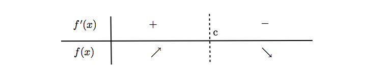
From now on, an increasing function, $f (x)$, is also denoted by $\color{brown}{f \nearrow}$ and decreasing denoted by $\color{brown}{f \searrow}$.
Theorem
If $f' (x) \geqslant 0$ for all $x \in (a, b)$ with $f' (x) = 0$ only at isolated points, then $f (x)$ is increasing on $[a, b]$. And if $f' (x) \leqslant 0$ for all $x \in (a, b)$, then $f (x)$ is decreasing.
The points at which $f' (x) = 0$ is very important in mathematical analysis:
Definition
The points of x at which $f' (x) = 0$ or nonexistencs are called critical points of $f (x)$.
Example
Determine the intervals at which the following functions are increasing or decreasing:
a). $x (20 - x)$
b). $2 x^3 + 3 x^2 - 12 x + 1$
c). $x^{- 2 / 3}$
Sol:
a) Since $f' (x) = 20 - 2 x$, there is only one critical point at $x = 10$. Therefore $f' (x) > 0$ for $x < 10$,
 this implies $f (x)$ is increasing and $f (x)$ is decreasing if $x > 10$.
b). $f' (x) = 6 x^2 + 6 x - 12 = 6 (x + 2) (x - 1) = 0$ implies $x = - 2$ or $1$. And

This implies $f (x)$ is increasing for $x < - 2$ or $x > 1$ and $f (x)$ is decreasing if $- 2 < x < 1$.
c). Since $f' (x) = - 2 x^{- 5 / 3} / 3 > 0$ for $x < 0$, $f (x)$ is increasing for $x < 0$ and decreasing for $x > 0$.

Example
Determine the intervals at which $f(x)=x^3-3x^2+2$ is increasing or decreasing.
Since $f'(x)=3x(x-2)$,
- $x\le0$ or $x\ge2$ implies $f'(x)\ge0$: $f(x)$ is increasing;
- $0\le x\le2$ implies $f'(x)\le0$: $f(x)$ is decreasing.
import numpy as np
import matplotlib.pyplot as plt
import mjsplot.mjsplot as mplt
import numpy as np
from numpy import sin,pi

%matplotlib inline
x=np.linspace(-5,5,101)
with plt.xkcd():
   plt.plot(x,x**3-3*x**2+2)
   plt.plot([0,0],[-50,50],'r--')
   plt.plot([2,2],[-50,50],'r--')
   plt.text(0.7,10, r'$\searrow$',size=20)
   plt.text(2.5,10, r'$\nearrow$',size=20)
   plt.text( -2,10, r'$\nearrow$',size=20)
   plt.ylim(-50,50)

Example
$x^4-4x^3+12$ $f'(x)=0$ implies $x=0,3$
$15x^{2/3}-3x^{5/3}$: critical points: $2,0$.
def critivalVal(x,func):
    sol=np.solve(func,x)
    return sol
from sympy import Symbol,solve,diff
def critivalVal(x,func):
    sol=solve(diff(func,x),x)
    return sol
x=Symbol("x")
fA=x**4-4*x**3+12
criticalA=critivalVal(x,fA)
print(criticalA)
[0, 3]
solve(diff(fA,x)>0)
And(3 < x, x < oo)
import numpy as np
import matplotlib.pyplot as plt
%matplotlib inline
x=np.linspace(-2,5,101)
with plt.xkcd():
  plt.plot(x,x**4-4*x**3+12)
  plt.plot([0,0],[-20,140],'r--')
  plt.plot([3,3],[-20,140],'r--')
  plt.ylim(-20,140)

x=Symbol("x")
fA=15*x**(2/3)-3*x**(5/3)
criticalA=critivalVal(x,fA
                     )
print(criticalA)
[2.00000000000000]
solve(diff(fA,x)>0)
And(0.0 < x, x < 2.0)
However, the critical value also includes $x=0$.
Note
Pthon could not recognize correct for $x^r$, for $x\le0$. To make the picture concern the odd root function can use parametric method:
$$ y= f(x)=15x^{2/3}-3x^{5/3}\Rightarrow (x,y)=(t^3,15t^2-3t^5)$$x=np.linspace(0,4,101)
t=np.linspace(-2**(1/3),0,101)
with plt.xkcd():
plt.plot(x,15*x**(2/3)-3*x**(5/3))
plt.plot(t**3,15*t**2-3*t**5,'b--')
plt.plot([0,0],[0,35],'r--')
plt.plot([2,2],[0,35],'r--')
plt.ylim(0,35)

Exercise, p 273
Find out the intervals on which $f(x)$ is increasing or decreasing and find out relative extrema if any.
24. $f(x)=x/(x-1)$
26. $f(x)=x\sqrt{4-x}$
30. $f(x)=x/\sqrt{x^2-1}$
36. $f(x)=\sin(x)/(1+\sin^2x)$, $x\in[0,2\pi)$
64 Show the following function is not monotonic in any interval , at which containing the origin:
68. (Yes or No) If both $f(x),g(x)$ are increasing, then $f(x)g(x)$ is also increasing.
70. (Yes or No) If $f(x)$ is increasing on interval $I=[a,b]$, then $f'(x)\ge0$ for $x\in(a,b)$.
eps=1e-6
x=np.linspace(1+eps,3,101)
t=np.linspace(-1,1-eps,101)
with plt.xkcd():
  plt.title(r' $n^\circ 24). x/(x-1)$',size=20)
  plt.plot(x,x/(x-1))
  plt.plot(t,t/(t-1),'b-')
  plt.plot([1,1],[-30,35],'r--')
  #plt.plot([2,2],[0,35],'r--')
  plt.ylim(-30,30)

import sympy
t=Symbol("t")
solve(diff(t*sympy.sqrt(4-t),t),t)
[8/3]
solve(diff(t*sympy.sqrt(4-t),t)>0)
And(-oo < t, t < 8/3)
x=np.linspace(-2,4,101)
with plt.xkcd():
  plt.title(r' $n^\circ 26). x\sqrt{4-x}$',size=20)
  plt.plot(x,x*np.sqrt(4-x))
  plt.plot([8/3,8/3],[-30,35],'r--')
  #plt.plot([2,2],[0,35],'r--')
  plt.ylim(0,3.5)

solve(diff(t/sympy.sqrt(t**-1),t),t)
[]
eps=1e-6
x=np.linspace(1+eps,2,101)
t=np.linspace(-2,-1-eps,101)
with plt.xkcd():
  plt.title(r' $n^\circ 30). x/\sqrt{x^2-1}$',size=20)
  plt.plot(x,x/np.sqrt(x**2-1))
  plt.plot(t,t/np.sqrt(t**2-1),'b-')
  #plt.plot([1,1],[-30,35],'r--')
  #plt.plot([2,2],[0,35],'r--')
  plt.ylim(-5,5)

from sympy import sin,pprint
t=Symbol("t")
pprint(diff(sin(t)/(1+sin(t)**2),t))
pprint(solve(diff(sin(t)/(1+sin(t)**2),t),t))
                   2
   cos(t)     2⋅sin (t)⋅cos(t)
─────────── - ────────────────
   2                        2
sin (t) + 1    ⎛   2       ⎞
               ⎝sin (t) + 1⎠
⎡-π   π⎤
⎢───, ─⎥
⎣ 2   2⎦
eps=1e-6
x=np.linspace(0,2*np.pi,101)

with plt.xkcd():
  plt.title(r' $n^\circ 36). \sin x/(1+\sin^2x)$',size=20)
  plt.plot(x,np.sin(x)/(1+np.sin(x)**2))
  plt.plot([np.pi/2,np.pi/2],[-30,35],'r--')
  plt.plot([3*np.pi/2,3*np.pi/2],[-30,35],'r--')
  #plt.plot([2,2],[0,35],'r--')
  plt.ylim(-.52,.52)

x=np.linspace(-.01,.01,4001)
mplt.plot(x,x/2+x**2*sin(1/x))

mplt.xlabel('x')
mplt.ylabel('y')
mplt.title(' 64). x/2 + x**2 sin(1/x)')

mplt.useDefaults()

mplt.setStyle("color_fg","#222")
mplt.setStyle("line_thickness",1)
mplt.setStyle("graph_line_thickness",1)
#mplt.setStyle("scaling_factor",1.1)
mplt.setStyle("color_bg","white")
mplt.grid(True)
mplt.save('testgraph', width='100%', height='300px')
/Users/cch/anaconda/lib/python3.5/site-packages/ipykernel/__main__.py:2: RuntimeWarning: divide by zero encountered in true_divide
  from ipykernel import kernelapp as app
/Users/cch/anaconda/lib/python3.5/site-packages/ipykernel/__main__.py:2: RuntimeWarning: invalid value encountered in sin
  from ipykernel import kernelapp as app
- For $x\to0^+$, take $x_n,x_{n+1}=\frac{1}{2n\pi},\frac{1}{2n\pi+\pi/2}$, where $n=1,2,3,\cdots$; $\{x_n\}\to0^+$.
- $f'(x_n)=1/2-1<0$, $f'(x_{n+1})=1/2+\frac{2}{2n\pi+\pi/2}>0$, i.e. $f(x)$ is increasing around $x_n$ but decrasing $x_{n+1}$ whatever $n$ is. This implies $f(x)$ could not be monotonic within $[x_{n+1},x_n]$.
- Similar for $x<0$.
x=np.linspace(-2,2,101)

with plt.xkcd():
  plt.title(r' $n^\circ 68). f,g$ increasing',size=20)
  plt.plot(x,x,label=r"$f=x$")
  plt.plot(x,x**3,label=r"$g=x^3$")
  plt.plot(x,x**4,label=r"$fg=x^4$")
  plt.legend(loc="best")
  plt.ylim(-8,8)

x=np.linspace(0,1,101)
t=np.linspace(-1,0,101)
with plt.xkcd():
  plt.title(r' $n^\circ 70). x^{1/3}$',size=20)
  plt.plot(x**3,x)
  plt.plot(t**3,t,'b-')
  plt.plot([0],[0],'r--')
  plt.plot([0,0],[-1,1],'r--')

Relative Minima and Maxima
Definition
Suppose that $f (x)$ is continuous on an interval, $I$.
- $f (c)$ is called a
relative minimum if there exists a neighborhood $N \subseteq I$ at $x=c$ and $f (c) \leqslant f (x)$ for all $x \in N$.
- $f (d)$ is called a relative
maximum if there exists a neighborhood $N \subseteq I$ of $x=d$ and $f (d) \geqslant f (x)$ for all $x \in N$.
If $f (c) \leqslant f (x)$ for all $x \in I$, then $f (c)$ is called the absolute minimum. If $f (d) \geqslant f (x)$ for all $x \in I$, then $f (d)$ is called the absolute maximum.
Theorem
(Existence of Extrema) If $f (x)$ is continuous on a close interval, then it attains both its absolute maximum and its absolute minimum.
From the definition of extrema, absolute extrema are also the relative extrema, but not necessary right conversely. The above theorem assures the the existence of absolute extrema but finding the relative is more complex.
Theorem
Suppose that $f (x)$ is continuous on an interval, $I$, and there is a relative extremum at $x = c$. Then
- $f' (c) = 0$, or
- $f' (c)$ fails to exist.
Such points are called critical points of $f (x)$ on the interval, $I$.
From tis theorem, only to check the values at critical points for relative extrema since it is only possible for at which $f (x)$ occurs relative minimum or maximum.
Example
Suppose that $f (x) = x - 3x^{1 / 3} $ for $x \in [- 2, 2] = [- 2, 0] \cup [0, 2]$.
- crititical points:
- $f(\pm2)=\pm2\mp3\cdot2^{1/3}, f(-1)=2,f(1)=-2$ and $f(0)=0$ implies maximum is 2 and minimun is $-2$.
%matplotlib inline
import numpy as np
import matplotlib.pyplot as plt
t=np.linspace(-2**(1/3),2**(1/3),101)
x=t**3
y=t**3-3*t
plt.plot(x,y)
[<matplotlib.lines.Line2D at 0x1084e2518>]

Example
$f (2) = 8$ is the maximum and $f (1) = - 9$ is the minimum for $f (x) = 3x^4- 4x^3 - 8$ in $[- 1, 2]$.
Analysis
- find out critical values:
- evaluate the function values at critical points, $x = - 1, 0, 1, 2$:
- $f (2) = 8$ is the absolute maximum and $f (1) = - 9$ is the absolute minimum of $f (x)$ on $[- 1, 2]$.
x=np.linspace(-1,2,101)
y=3*x**4-4*x**3-8
plt.plot(x,y)
plt.grid()

Example
Find all the extreme values of $f (x) = 2 \cos x-x$ for $x \in [0, 2\pi]$.
- critical values:
- $f(0)=2,f(\frac{7\pi}{6})\sim -5.4, f(\frac{11\pi}{6})\sim -4.03,f(2\pi)=2-2\pi$ implies absolute maximum at $x=0$ and absolute minimum at $\frac{7\pi}{6}$
from numpy import cos,pi
x=7/6*pi
2*cos(x)-x
-5.3972422367569699
x=11/6*pi
2*cos(x)-x
-4.0275357240124103
x=np.linspace(0,2*pi,101)
with plt.xkcd():
   plt.title(r"2cos x-x")
   plt.plot(x,2*cos(x)-x)
   plt.xlim(0,2*pi)
   plt.axis("equal")
   plt.grid(True, lw=0.5, zorder=0)

Example
Find all the extreme values of $f (x) = 2 \sin x+\sin2x$ for $x \in [0, 3\pi/2]$.
- critical values:
i.e. $x=\pi/3,\pi$.
- $f(0)=0,f(\frac{\pi}{3})=3\sqrt3/2, f({\pi})=0,f(3\pi/2)=-2\pi$ implies absolute maximum at $x=\pi/3$ and absolute minimum at $\frac{3\pi}{2}$
from numpy import sin
x=np.linspace(0,3*pi/2,101)
plt.plot(x,2*sin(x)+sin(2*x))
plt.xlim(0,3*pi/2)
plt.axis("equal")
plt.grid()

Exercise, p253
38). Find out all the critical values of $4t^{1/3}+3t^{4/3}$ and extremum if any.
1.
$$ f'(t)=\left(4t^{\frac{1}{3}}+3t^{\frac{4}{3}}\right)'=\frac{4}{3}\left(t^{-\frac{2}{3}}+3t^{\frac{1}{3}}\right) =\frac{4(1+3t)}{3t^\frac{2}{3}} $$a). If $f'(t)=0\Rightarrow1+3t=0\to t=-1/3$
b). If $f'(t)=0$ fails to exist, then the denominator is zero, $t^{2/3}=0\to t=0$
2. Since
$$\lim\limits_{t\to\pm\infty} f(t) =+\infty,$$
$f(t)$ can only attain its absolute minimum. The minimum is $f(-1/3)$, which is smaller than 0, since it is smaller than $f(0)=0$.
x=np.linspace(-1,1,101)
t= x**3
y= 4*x+3*x**4
with plt.xkcd():
     plt.plot(t,y)
     plt.plot((0,0),(-4,8),"r--")
     plt.plot((-(1/3),-(1/3)),(-4,8),"r--")
     plt.grid(True, lw=0.5, zorder=0)

x=np.linspace(-2,2,101)

y= x**2/(1+x**2)
with plt.xkcd():
     plt.plot(x,y)
     plt.grid(True, lw=0.5, zorder=0)
     #plt.plot((0,0),(-4,8),"r--")
     #plt.plot((-(1/3),-(1/3)),(-4,8),"r--")

Exercise
40). Find out all the critical values of $\frac{x^2}{x^2+1}$.
$$ f'(x)=\left(1-\frac{1}{1+x^2}\right)'=\frac{2x}{(1+x^2)^2} $$If $f'(x)=0\Rightarrow x=0$.
42). Find out all the critical values of $2\sin{x}-\cos{2x}$.
\begin{eqnarray} 0= (2\sin{x}-\cos{2x})'&=& 2\cos x + (2\sin2x)\\ &=& 2(\cos x+2\sin\cos x)\\ &=& 2\cos x (2\sin x+1)\\ &\Downarrow&\\ && \cos x=0 \text{ or }\sin x=-1/2\\ x &=& n\pi+\pi/2, n\pi+(-1)^{n+1}\pi/6, \text{ where } n\in\mathbf{Z} \end{eqnarray}Exercise
50). Find out all the absolute extrema of $\frac{\sqrt u}{1+u^2}$ on $[0,2]$ if any.
$$ 0=f'(t)=\left(\frac{\sqrt u}{1+u^2}\right)'=\frac{1+u^2-4u^2}{2\sqrt u(1+u^2)^2} \to u=\frac{1}{\sqrt3} $$
$f(1/\sqrt3)=\frac{(1/3)^{1/4}}{1+1/3}$ is absolute maximum and $f(0)=0$ is the absolute minimum.
u=np.linspace(0,2,101)
with plt.xkcd():
    plt.plot(u,np.sqrt(u)/(1+u**2))
    plt.plot((1/np.sqrt(3),1/sqrt(3)),(0,0.6),'r--')
    plt.grid(True, lw=0.5, zorder=0)

from sympy import Symbol,solve,diff,sqrt,pprint
x=Symbol("x")
def critivalVal(x,func):
    sol=solve(diff(func,x),x)
    pprint(sol)
fA=sqrt(x)/(1+x**2)
criticalA=critivalVal(x,fA)
       3/2
    2⋅x             1
- ───────── + ─────────────
          2        ⎛ 2    ⎞
  ⎛ 2    ⎞    2⋅√x⋅⎝x  + 1⎠
  ⎝x  + 1⎠
56). Find out extremum of $f (x) = x \sqrt{4 - x^2}$ for $ x\in[0,2]$
- First find all its critical point(s):
It is obviously that $f (x)$ attains its maximum 2 at $x = \sqrt{2}$ and minimum 0 at $x=0,2$.
x=np.linspace(0,2,101)
with plt.xkcd():
    plt.plot(x,x*np.sqrt(4-x**2))
    plt.plot([np.sqrt(2),np.sqrt(2)],[0,2],'r--')
    plt.grid(True, lw=0.5, zorder=0)

Example
Find the critical points of the following functions and determine whether the extrema occur at these points:
- $f (x) = x^2 - 2 x$. Since
there is only one critical point, $x = 1$. And from the table
 It is obvious that $f (x)$ attains its (absolute) minimum at the critical
point, $x = 1$.
- $g (x) = x + \frac{1}{x}$, for $x \in (0, \infty)$. Since
\begin{eqnarray*}
& g' (x) = 0 & \\
\Longrightarrow & 1 - \frac{1}{x^2} = 0 & \\
\Longrightarrow & x = 1 &
\end{eqnarray*}
there is only one critical point, $x = 1$ and it is obvious that $g (x)$ attains its (absolute) minimum at the critical point, $x = 1$.
- $h (x) = x^{1 / 3}$. Since
\begin{eqnarray*}
& h' (x) = 0 & \text{or fails to exist}\\
\Longrightarrow & \frac{1}{3 x^{2 / 3}} = 0 & \text{or fails to exist}\\
\Longrightarrow & x = 0 &
\end{eqnarray*}
there is only one critical point, $x = 0$. And from the table
It is obvious that $f (x)$ attains its (absolute) minimum at the critical
point, $x = 1$.
- $g (x) = x + \frac{1}{x}$, for $x \in (0, \infty)$. Since
\begin{eqnarray*}
& g' (x) = 0 & \\
\Longrightarrow & 1 - \frac{1}{x^2} = 0 & \\
\Longrightarrow & x = 1 &
\end{eqnarray*}
there is only one critical point, $x = 1$ and it is obvious that $g (x)$ attains its (absolute) minimum at the critical point, $x = 1$.
- $h (x) = x^{1 / 3}$. Since
\begin{eqnarray*}
& h' (x) = 0 & \text{or fails to exist}\\
\Longrightarrow & \frac{1}{3 x^{2 / 3}} = 0 & \text{or fails to exist}\\
\Longrightarrow & x = 0 &
\end{eqnarray*}
there is only one critical point, $x = 0$. And from the table
 it is obvious that $h (x)$ is always increasing and this implies no
extremum for $h (x)$.
- $u (\theta) = \sin \theta + \cos \theta$, for $\theta \in [0, \pi]$.
Since
\begin{eqnarray*}
& u' (\theta) = 0 & \\
\Longrightarrow & \cos \theta - \sin \theta = 0 & \\
\Longrightarrow & \cos \theta = \sin \theta & \\
\Longrightarrow & \tan \theta = 1 & \\
\Longrightarrow & \theta = \frac{\pi}{4} &
\end{eqnarray*}
there is only one critical point, $x = 1$. And from the table
it is obvious that $h (x)$ is always increasing and this implies no
extremum for $h (x)$.
- $u (\theta) = \sin \theta + \cos \theta$, for $\theta \in [0, \pi]$.
Since
\begin{eqnarray*}
& u' (\theta) = 0 & \\
\Longrightarrow & \cos \theta - \sin \theta = 0 & \\
\Longrightarrow & \cos \theta = \sin \theta & \\
\Longrightarrow & \tan \theta = 1 & \\
\Longrightarrow & \theta = \frac{\pi}{4} &
\end{eqnarray*}
there is only one critical point, $x = 1$. And from the table
 it is obvious that $u (\theta)$ attains its (absolute) maximum at the
critical point, $\theta = \pi / 4$.
- $p (x) = x e^{- x}$, for $x \in [0, \infty)$. Since
\begin{eqnarray*}
& p' (x) = 0 & \\
\Longrightarrow & e^{- x} - x e^{- x} = 0 & \\
\Longrightarrow & (1 - x) e^{- x} = 0 & \\
\Longrightarrow & x = 1 &
\end{eqnarray*}
there is only one critical point, $x = 1$. And from the table
it is obvious that $u (\theta)$ attains its (absolute) maximum at the
critical point, $\theta = \pi / 4$.
- $p (x) = x e^{- x}$, for $x \in [0, \infty)$. Since
\begin{eqnarray*}
& p' (x) = 0 & \\
\Longrightarrow & e^{- x} - x e^{- x} = 0 & \\
\Longrightarrow & (1 - x) e^{- x} = 0 & \\
\Longrightarrow & x = 1 &
\end{eqnarray*}
there is only one critical point, $x = 1$. And from the table
 $p (x)$ attains its (absolute) maximum at point, $x = 1$.
3.1 Exercise
Find the critical points of the following functions and determine whether the extrema occur at these points:
- $x^3 + 3 x$+1
- 2$\sin x + \sin 2 x$ for $x \in [0, \pi]$
- $x^2 e^{- x / 2}$ for $x \in [0, \infty)$
Sol
- $f (x) = x^3 + 3 x$+1. Since \begin{eqnarray*} & f' (x) = 0 & \\ \Longrightarrow & 3 x^2 + 3 > 0 & \end{eqnarray*} there is no any critical point and it is always increasing since the derivative is povitive for all $x$.
- $u (x) = \text{2} \sin x + \sin 2 x$, for $x \in [0, \pi]$. Since
Since $\pi$ is also one of endpoints, there is only one critical point, $x = \pi / 3$. And from the table
 it is obvious that $u (x)$ would attain its (absolute) maximum at the
critical point, $x = \pi / 3$.
- $p (x) = x^2 e^{- x / 2}$, for $x \in [0, \infty)$. Since
\begin{eqnarray*}
& p' (x) = 0 & \\
\Longrightarrow & 2 x e^{- x / 2} - x^2 e^{- x / 2} / 2 = 0 & \\
\Longrightarrow & (2 - \frac{x}{2}) x e^{- x} = 0 & \\
\Longrightarrow & x = 4 &
\end{eqnarray*}
it is obvious that $u (x)$ would attain its (absolute) maximum at the
critical point, $x = \pi / 3$.
- $p (x) = x^2 e^{- x / 2}$, for $x \in [0, \infty)$. Since
\begin{eqnarray*}
& p' (x) = 0 & \\
\Longrightarrow & 2 x e^{- x / 2} - x^2 e^{- x / 2} / 2 = 0 & \\
\Longrightarrow & (2 - \frac{x}{2}) x e^{- x} = 0 & \\
\Longrightarrow & x = 4 &
\end{eqnarray*}there is only one critical point, $x = 4$. And from the table
 $p (x)$ attains its (absolute) maximum at point, $x = 4$.
Theorem
(First Derivative Test) Suppose that $f (x)$ is continuous on interval, $I$, containing $c$, and differentiable in I, possibly except $x = c$. Then
a). If the sign of $f' (x)$ from the left side $x = c$ to to the right side changes from positive to negative, $f (c)$ is a relative maxima.
b). If the sign of $f' (x)$ from the left side $x = c$ to to the right side changes from negative to positive, $f (c)$ is a relative minimum.
 **c).** If the sign of the $f' (x)$ does not't change the sign about $x =
c$, $f (c)$ is not a relative extremum.
**c).** If the sign of the $f' (x)$ does not't change the sign about $x =
c$, $f (c)$ is not a relative extremum.
Example
Suppose that $f (x) = x \ln x$ for $x \in (0, \infty)$. First find out all the critical point(s) of $f (x)$: \begin{eqnarray*} & f' (x) = 0 & \\ \Longrightarrow & \ln x + 1 = 0 & \\ \Longrightarrow & x = e^{- 1} & \end{eqnarray*} there is only one critical point, $x = e^{- 1}$. And from the table

the sign of $f' (x)$ changes from negative to positive at $x = e^{- 1}$. This means that $f (e^{- 1}) = - e^{- 1}$ is relative minimum of $f (x)$.
Example
Suppose that $f (x) = 1 / (1 + x^2)$ for $x \in \mathbb{R}$. First find out all the critical point(s) of $f (x)$: \begin{eqnarray*} & f' (x) = 0 & \\ \Longrightarrow & \frac{- 2 x}{(1 + x^2)^2} = 0 & \\ \Longrightarrow & x = 0 & \end{eqnarray*} there is only one critical point, $x = 0$. And from the table

the sign of $f' (x)$ changes from positive to negative at $x = 0$. This means that $f (0) = 1$ is relative maximum of $f (x)$.
Example
(Sample Mean) Suppose that $x_i, i = 1, 2, \cdots, n$ are $n$ known data. Also define
$$F (x) = \sum^n_{i = 1} (x - x_i)^2\text{ for }x \in \mathbb{R}$$.
Then the critical point of $F (x)$ can be found out by the following:
\begin{eqnarray*} & F' (\hat x) = 0 & \\ \Longrightarrow & \sum^n_{i = 1} 2 (\hat x - x_i) = 0 & \\ & \Downarrow & \\ & \sum^n_{i = 1} \hat x = \sum^n_{i = 1} x_i & \\ \Longrightarrow & n \hat x = \sum^n_{i = 1} x_i & \\ \Longrightarrow & \hat x = \frac{1}{n} \sum^n_{i = 1} x_i & \end{eqnarray*}there is only one critical point,
$$\hat x=\frac{1}{n} \sum^n_{i = 1} x_i,$$or called sample mean, denoted as $\bar{x}$. And from the table

the sign of $F' (x)$ changes from negative to positive at $x = \bar{x}$ from left to right. This means that $F (\bar{x})$ is relative minimum of $F (x)$.
Concavity and Inflation Points
Definition
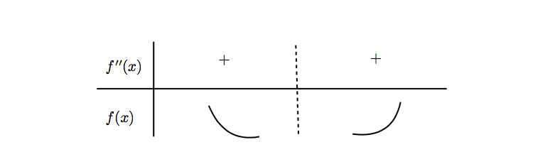
$f (x)$ is called concave upward if $f' (x)$ is increasing and $f (x)$ is
called concave downward if $f' (x)$ is decreasing. And the point, at which the concavity changes, is called
inflation of curve.
Theorem
$f (x)$ is called concave upward if $f'' (x) > 0$ and $f (x)$ is called concave downward if $f'' (x) < 0$.
Proof Since $f'' (x) > 0$ implies $f' (x)$ is increasing. Therefore $f (x)$ is concave upward.

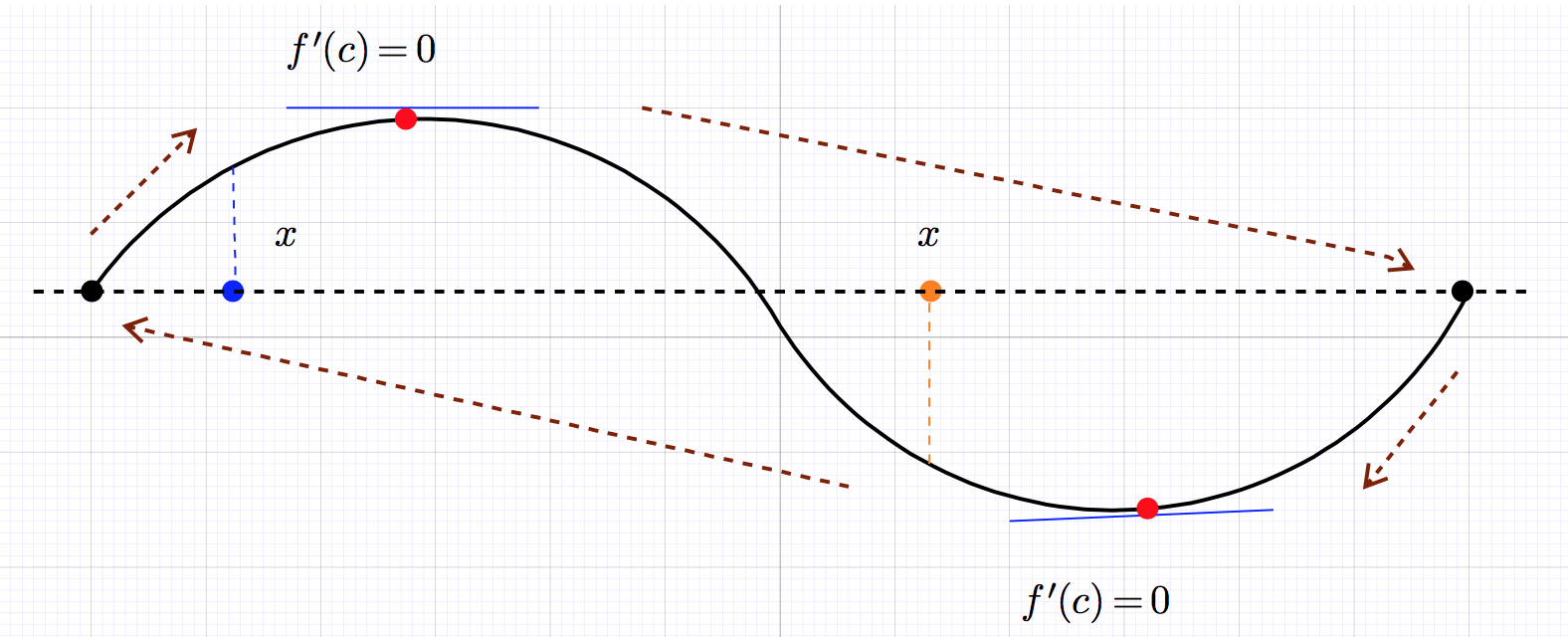
According the sign of $f' (x)$ and $f'' (x)$, the graphs of functions can be one of four kinds:

Theorem
(Second Derivatives Test): Suppose that $f (x)$ is differentiable on an open interval, $I$ containing $x = c$ in which $f' (c) = 0$ and $f'' (x)$ exists for all the $x \in \overset{\circ}{I}$. Then
a). If $f'' (c) < 0$, then $f (x)$ is a relative maximum.
 b). If $f'' (c) > 0$, then $f (x)$ is a relative minimum.
c). If $f'' (c) = 0$, no conclusion.
Example
Suppose that $f (x) = x^4 - 4 x^3 + 12$.
- critical values
there are two critical points, $x = 0, 3$: 2. Concavity, \begin{eqnarray*} 0 & = & f'' (x)\\ & = & 12 x^2 - 24 x=12x(x-2)\\ \Longrightarrow & & x = 0 \text{ and } 2 \end{eqnarray*}
  f'(x)  |       -          |  +
 ------------ 0 ------2-----3--------
  f''(x) |  + |   -   |     +
This means $f(x)$ is concave upward for $x\in(-\infty,0]\cup[2,\infty)$ and downward otherwise.
x=np.linspace(-2,4,101)
t=np.linspace(0,2,101)
plt.plot(x,x**4-4*x**3+12)
plt.plot(t,t**4-4*t**3+12,'r-')
plt.plot([0,0],[-20,60],color="brown")
plt.plot([2,2],[-20,60],color="brown")
plt.text(0.5,40,"$f''(x)<0$",size=16)
plt.text(-1.4,50,"$f''(x)>0$",size=16)
plt.text(2.4,30,"$f''(x)>0$",size=16)
<matplotlib.text.Text at 0x10a3cdb70>

Example
Suppose that $f (x) = x^4 - 8 x^2 + 2$. Then $f (x)$ attains it relative extrema as follows:
Since \begin{eqnarray*} 0 & = & f' (x)\\ & = & 4 x^3 - 16 x\\ \Longrightarrow & & x = 0 \text{ and } \pm 2 \end{eqnarray*} there are three critical points, $x = 0, 2, - 2$:
- $f (0) = 2$ is relative maximum since $f' (0) = 0$ and $f'' (0) = - 16 < 0$.
- $f (\pm 2) = - 14$ are relative minima since \ $f' (\pm 2) = 0$ and $f'' (\pm 2) = 32 > 0$
Example
Consider the Cost function, $C (x) = 500 + 20 x + 5 x^2$ for $x > 0$. Define the average cost funtion and marginal cost function as follows: \begin{eqnarray*} \bar{C} & = & C (x) / x = 20 + 5 x + 500 / x\\ \text{MC} & = & C' (x) = 20 + 10 x \end{eqnarray*} Since \begin{eqnarray*} \bar{C}' = 5 - 500 / x^2 = 0 & \Rightarrow & x = 10\\ \text{MC}' (= 10) = 0 & \Rightarrow & \text{ No solution} ! \end{eqnarray*} $\bar{C}$ has only one critical value at $x = 10$ and $\bar{C}'' > 0$. Then ${\bar{C} (10)}$ is the relative minimum. It is also be the absolute minimum for ${\bar{C} (x)}$ in $(0, \infty)$. But there is no extrema.since MC is always increasing (to $+\infty$).
Example
Plot the graph of $f (x) = x \sqrt{1 - x^2}$ for $0\le x\le 1$ and discuss its extrema .
- First find all its critical point(s):
- Discuss its monotoncity and concavity:
Then
 - connect the sub graphs at: $f (0) = f (1) = 0$ and $f (1 / \sqrt{2})
= 1 / 2$, ref the following:
- connect the sub graphs at: $f (0) = f (1) = 0$ and $f (1 / \sqrt{2})
= 1 / 2$, ref the following:
It is obviously that $f (x)$ attains its maximum 1/2 at $x = \frac{1}{\sqrt{2}}$.
%matplotlib inline
import matplotlib.pylab as plt
import numpy as np
from numpy import sqrt,pi,sin,cos,exp
x=np.linspace(0,1,101)
plt.plot(x,x*sqrt(1-x**2))
[<matplotlib.lines.Line2D at 0x108afd940>]

Example
Plot the graph of $f (x) = x - \sin x$ for $x \in [0, \pi]$. And find all the zero root of $f (x)$.
Since $f (x)$ is odd, i.e. $f (- x) = - f (x)$, its graph is symmetry with repect to the original $(0.0)$. Therefore, only need to consider the part for $x > 0$.
- Since $| \cos x| \leqslant 1$, it is trivial that
This implies that $f (x)$ is always increasing.
- Concavity:
implies that it is always concave upward!
Then
 Also note $f (0) = 0 - \sin 0 = 0$ and increasing always $\Rightarrow$ there
is no any $x > 0$ such that $f (x) = 0$!
Also note $f (0) = 0 - \sin 0 = 0$ and increasing always $\Rightarrow$ there
is no any $x > 0$ such that $f (x) = 0$!
x=np.linspace(0,pi,101)
plt.plot(x,x-sin(x))
[<matplotlib.lines.Line2D at 0x108c23198>]

Exercise
plot the graphs of the following functions:
- $f (x) = x e^{- x}$, $x \in [0, \infty)$
- $g (x) = x^3 + x^2 - x + 3$
x=np.linspace(0,10,101)
t=np.linspace(-5,5,101)
f=x*exp(-x)
g=t**3+t**2-t+3
plt.subplot(211)
plt.plot(x,f)
plt.subplot(212)
plt.plot(t,g)
[<matplotlib.lines.Line2D at 0x108d52908>]

3.4 Exercises
18. Decide the concavity of $f(x)=x-\sqrt{1-x^2}$
Since $$f''(x)=\frac{-1}{(1-x^2)^{3/2}}<0$$ $f(x)$ is always concave downward for $|x|\le1$.
import sympy
from sympy import Symbol,sqrt,diff,solve,pprint,cos,sin
x= Symbol("x")
f=x-sqrt(1-x**2)
pprint(diff(f,x,2))
     2
    x
 ──────── + 1
    2
 - x  + 1
─────────────
   __________
  ╱    2
╲╱  - x  + 1
28. Decide the concavity of $f(x)=x-\sin x$ for $x\in[0,4\pi]$.
Since $$f''(x)=\sin(x)$$ $f(x)$ is concave downward for $x\in [\pi,2\pi]\cup[3\pi,4\pi]$ and concave upward for $x\in [0,\pi]\cup[2\pi,3\pi]$.
x= Symbol("x")
f=x-sin(x)
pprint(diff(f,x,2))
sin(x)
32. Decide the concavity of $f(x)=\frac{\sin x}{1+\sin x}$ for $x\in[-\pi/2,3\pi/2]$.
Since $$f''(x)=-\frac{\sin^2x+\sin x+2\cos^2x}{(1+\sin x)^3}=-\frac{2+\sin x-\sin^2x}{(1+\sin x)^3}=-\frac{2-\sin x}{(1+\sin x)^2}\le0$$ $f(x)$ is always concave downward.
f=1-1/(1+sin(x))
pprint(diff(f,x,2))
 ⎛              2    ⎞
 ⎜         2⋅cos (x) ⎟
-⎜sin(x) + ──────────⎟
 ⎝         sin(x) + 1⎠
───────────────────────
                 2
     (sin(x) + 1)
with plt.xkcd():
     x=np.linspace(-np.pi/2,3*np.pi/2,101)
     plt.plot(x,np.sin(x)/(1+np.sin(x)))
     plt.ylim(-5,1)
/Users/cch/anaconda/lib/python3.5/site-packages/ipykernel/__main__.py:3: RuntimeWarning: divide by zero encountered in true_divide
  app.launch_new_instance()

36. Find out inflation point of $f(x)=\cos\sin x$ for $x\in(-2,2)$.
Since $$f''(x)=\sin x \sin\sin x -\cos^2x\cos\sin x$$ Not tritial to decide the concavity of $f(x)$.
f=cos(sin(x))
pprint(diff(f,x,2))
                        2
sin(x)⋅sin(sin(x)) - cos (x)⋅cos(sin(x))
# Failed by SymPy
solve(diff(f,x,2),x)
with plt.xkcd():
     from numpy import sin,cos
     x=np.linspace(-2,2,101)
     plt.plot(x,cos(sin(x)))
     plt.plot(x,sin(x)*sin(sin(x))-cos(x)**2*cos(sin(x)))
     #plt.ylim(-5,1)

Newton's Method
$$X_{n+1}=x_n-\frac{f(x_n)}{f'(x_n)}$$
from scipy.optimize import fsolve
from numpy import sin,cos
def pfunc(x)
    return -cos(x)*sin(sin(x))
def ppfunc(x):
        return sin(x)*sin(sin(x))-cos(x)**2*cos(sin(x))
def x1(x)
    return x-cos(sin(x))/pfunc(x)
def f(x):
    return sin(x)*sin(sin(x))-cos(x)**2*cos(sin(x))

def df(x):
    return cos(x)*sin(sin(sin(x)))+sin(x)*cos(x)*cos(sin(x))+2*sin(x)*cos(x)*cos(sin(x))+cos(x)**3*sin(sin(x))
def dx(f, x):
    return abs(0-f(x))

def newtons_method(f, df, x0, e):
    delta = dx(f, x0)
    while delta > e:
        x0 = x0 - f(x0)/df(x0)
        delta = dx(f, x0)
    print('Root is at: ', x0)
    print('f(x) at root is: ', f(x0))
x0s = [-1., 1]
for x0 in x0s:
    newtons_method(f, df, x0, 1e-5)
Root is at:  -0.742660403252
f(x) at root is:  -7.65244390316e-06
Root is at:  0.742660403252
f(x) at root is:  -7.65244390316e-06
x1=1-f(1)/df(1);x1
0.68925003110856475
x2=x1-f(x1)/df(x1);x2
0.74291846769037984
with plt.xkcd(False):
     from numpy import sin,cos
     x=np.linspace(-2,2,101)
     plt.plot(x,cos(sin(x)))
     plt.plot(x,sin(x)*sin(sin(x))-cos(x)**2*cos(sin(x)))
     x0=1
     plt.plot([1,1,x1,x1,x2,x2],[0,f(1),0,f(x1),0,f(x2)])
     plt.plot([-2,2],[0,0],'k--')
     plt.xlim([0.6,1.1])
     plt.ylim([-0.5,0.5])
     plt.text(1,0-0.05,"$x_0$")
     plt.text(x1,0+0.05,"$x_1$")
     plt.text(x2,0-0.05,"$x_2$")
     plt.text(x0,0,"x",color="red")
     plt.text(x1,0,"x",color="red")
     plt.text(x2,0,"x",color="red")
     #plt.plot([x0,x0,x1],[0,ppfunc(x0)])

fsolve(func,[-np.pi/2,3*np.pi/2])
array([ 1310.78680103, -124.92104166])
fsolve(func,-1)
array([-0.74266448])
fsolve(func,1)
array([ 0.74266448])
42. Find out relative extema of $f(t)=t^2+1/t$ if any.
- $f'(t)=2t-1/t^2$ implies only one critical point, $t_0=1/2^{1/3}$;
- $f''(t)=2+2/t^3$ and $f''(t_0)>0$ implies $f(t)$ attains its relative minimum at $t_0$.
with plt.xkcd():
     from numpy import sin,cos
     x=np.linspace(0.01,4,101)
     plt.plot(x,x**2+1/x)
     #plt.plot(x,sin(x)*sin(sin(x))-cos(x)**2*cos(sin(x)))
     plt.ylim(0,10)

44. Find out relative extema of $f(x)=x\sqrt{4-x^2}$ if any.
- $f'(x)=\frac{4-2x^2}{\sqrt{4-x^2}}$ implies only one critical point, $x_0=\sqrt2$;
- $f''(x)=-\frac{x(12-2x^2)}{\sqrt{(4-x^2)^{3/2}}}$ and $f''(x_0)<0$ implies $f(x)$ attains its relative maximum at $x_0$ and is also its maximum.
from sympy import sqrt
x=Symbol("x")
f=x*sqrt(4-x*x)
pprint(diff(f,x,2))
   ⎛    2       ⎞
   ⎜   x        ⎟
-x⋅⎜──────── + 3⎟
   ⎜   2        ⎟
   ⎝- x  + 4    ⎠
──────────────────
     __________
    ╱    2
  ╲╱  - x  + 4
with plt.xkcd():
     from numpy import sin,cos ,sqrt
     x=np.linspace(0,4,101)
     plt.plot(x,x*sqrt(4-x**2))
     #plt.plot(x,sin(x)*sin(sin(x))-cos(x)**2*cos(sin(x)))
     plt.ylim(0,10)
/Users/cch/anaconda/lib/python3.5/site-packages/ipykernel/__main__.py:4: RuntimeWarning: invalid value encountered in sqrt

68. $f(x)=x|x|$ has a inflation at $(0,0)$ but $f''(0)$ fails to exist.
- Similar to 2, $f_{-}''(0)=-2\ne f''_+(0)$; theirfor $f''(0)$ fails to exist.
76. Suppose that $f'(a)=f''(a)=0$ but $f'''(a)\ne0$. Then $f(x)$ has a inflation point at $(a,f(a))$.
With of loss generality, we assume $f'''(a)>0$. Since $f''(a)=0$$, we have:
$$ f'''(a)=\lim_{h\to0}\frac{f''(a+h)-f''(a)}{h}=\lim_{h\to0}\frac{f''(a+h)}{h}>0$$
Then there exist a small $h_0>0$ such that
$$\frac{f''(a+h)}{h}>0\text{ for any } |h|<h_0$$a). if $0<h<h_0$, $f''(a+h)>0$;
b). if $-h_0<h<0$, $f''(a+h)<0$;
Thus the second derivative changes sign from negative to positive while $x$ moves from left to right of $x=a$. This proves that $f(x)$ has an inflation point at $(a,f(a))$.
Suppose $f(x)=\cos x-1+x^2/2-x^3/6$.
- $f'(0)=\left.-\sin x +x -x^2/2\right|_{x=0}=0$,
- $f''(0)=\left.-\cos x +1 -x\right|_{x=0}=0$,
- $f'''(0)=\left.\sin x -1\right|_{x=0}=-1\ne0$,
Then $f(x)$ has an inflation at $(0,0)$
x=np.linspace(-1,1,101)
plt.plot(x, cos(x)-1+x**2/2-x**3/6)
[<matplotlib.lines.Line2D at 0x109e3d470>]

Finding Absolute Extrema
Note
Procedure for finding Extrema: Suppose that $f (x)$ is continuous on $[a,b]$.
i). Find out all the critical values.
ii). Compute the values $f (a), (b)$ and the $f (c)$ where $c$ is the critical values.
iii). Absolute maximum of $f (x)$ is the largest in ii). and absolute minimum is the smallest in ii).
Example
$f (8) = 133$ is the maximum and $f (4) = - 75$ is the minimum for $f (x) = x^3 - 3 x^2 - 24 x + 5$ in $[- 3, 8]$.
Analysis
- find out critical values:
- evaluate the function valus at critical points, $x = - 3, - 2, 4, 8$:
- $f (8) = 133$ is the absolute maximum and $f (4) = - 75$ is the absolute minimum of $f (x)$ on $[- 3, 8]$.
Example
$f (8) = 4$ is the maximum and $f (0) = 0$ is the minimum for $f (x) = x^{2/3}$ in $[- 1, 8]$.
Analysis
- find out critical values:
- evaluate the function valus at critical points, $x = - 1, 0, 8$:
- $f (8) = 4$ is the absolute maximum and $f (0) = 0$ is the absolute minimum for $f (x)$ in $[- 1, 8]$
Note
Procedure for finding Extrema II: Suppose that $f (x)$ is continuous on $(a,b)$.
i.) Find out all the critical values.
ii). Compute the values $\lim\limits_{x \rightarrow a^+} f (x), \lim\limits_{x \rightarrow b^-} f (x)$, if exists, and $f (c)$ where $c$ is the critical values.
iii). Absolute maximum of $f (x)$ is the largest $f (c)$ in ii) if $f (c) \geqslant \lim\limits_{x \rightarrow a^+} f (x) \text{ and } \lim\limits_{x \rightarrow b^-} f (x)$
iv). Absolute minimum of $f (x)$ is the smallest $f (c)$ in ii) if $f (c) \leqslant \lim\limits_{x \rightarrow a^+} f (x) \text{ and } \lim\limits_{x \rightarrow b^-} f (x)$.
Example
Finding the extrema for $f (x) = \frac{x}{1 - x^2}$ in $(- 1, 1)$ if any.
Since it is possible for $f (x)$ to approach $\pm \infty$ ( for example as $x \rightarrow 1^{\pm}$), $f (x)$ has no extrema.
Analysis
- find out critical point if any:
- No critical point and $f' (x) > 0 \Longrightarrow f (x) \nearrow$.
- Since $\lim\limits_{x \rightarrow - 1^+}\frac{x}{1 - x^2} = - \infty$ and $\lim\limits_{x \rightarrow 1^-} \frac{x}{1 - x^2} = \infty$, no any extrema exist!
Eexercise
Discuss the existence of extrema for a) $8 x^{1 / 3} - 2 x^{4 / 3}$ on $[- 1, 8]$, b) $\sqrt{x} (1 - x)$ on $[0, 4]$.
import matplotlib.pyplot as plt
import numpy as np
from numpy import abs,sqrt,sign
%matplotlib inline
x1=np.linspace(-1,8,101)
x2=np.linspace(0,4,101)
plt.plot([1,2,2])
plt.subplot(121)
plt.plot(x1,8*sign(x1)*(abs(x1))**(1/3)-2*abs(x1)**(4/3))

plt.subplot(122)
plt.plot(x2,sqrt(x2)*(1-x2))
[<matplotlib.lines.Line2D at 0x109385470>]

Analysis a).
- find out critical points: \begin{eqnarray*} 0 \text{ or fails to exist } & = & f' (x)\\ & = & \frac{8 (1 - x)}{3 x^{\frac{2}{3}}} \end{eqnarray*} implies that $0$ and 1 are the critical points.- $x = - 1, 0, 1, 8$ \begin{eqnarray*} f (- 1) & = & - 10\\ f (0) & = & 0\\ f (1) & = & 6\\ f (8) & = & - 16 \end{eqnarray*}
- the maximum is 6 and the minimum is $- 16$.
Since $f (x)$ is continuous on closed interval $[- 1, 8]$ and $f (- 1) = - 10, f (0) = 0, f (1) = 6, f (8) = - 16$, the maximum is 6 and the minimum is -16.
Analysis for b)
- find out critical points: \begin{eqnarray*} 0 \text{ or fails to exist} & = & \left( \sqrt{x} (1 - x) \right)'\\ & = & \frac{1 - 3 x}{2 \sqrt{x}}\\ \Rightarrow & & x = 0 \text{ and } \frac{1}{3} \end{eqnarray*} - $x = 0, 1 / 3, 4$: \begin{eqnarray*} f (0) & = & 0\\ f (1 / 3) & = & \frac{2}{3 \sqrt{3}}\\ f (4) & = & - 6 \end{eqnarray*} - The critical value is 1/3 and the boundary points are 0 and 4. Since $f (0) = 0, f (1 / 3) = \frac{2}{3 \sqrt{3}}$ and $f (4) = - 6$, maximum is $\frac{2}{3 \sqrt{3}}$ and minimum is -6.Rolle's Theorem and the Mean Value Theorem
Theorem (Rolle's Theorem)
Assume that $f (x)$ is continuous on $[a, b]$ and differentiable in $(a, b)$. If $f (a) = f (b)$, there exists at least $c \in (a, b)$ such that $f' (c) = 0$.
 Proof:
---
1. If $f (x)$ is constant on $[a, b]$, then done.
- Suppose that $f (x) > f (a) = C$ for some $x \in (a, b)$. By the
Extrema Value Theorem, $f (x)$ has a maximum for some $c \in (x, b)$.
Since $f (x) $ is differentiable in this interval, $f' (c) = 0$.
- Case about $f (x) < f (a) = C$ could be proved similarly.
Proof:
---
1. If $f (x)$ is constant on $[a, b]$, then done.
- Suppose that $f (x) > f (a) = C$ for some $x \in (a, b)$. By the
Extrema Value Theorem, $f (x)$ has a maximum for some $c \in (x, b)$.
Since $f (x) $ is differentiable in this interval, $f' (c) = 0$.
- Case about $f (x) < f (a) = C$ could be proved similarly.
Example
Suppose that $f (x) = x - x^{1 / 3} $ for $x \in [- 1, 1] = [- 1, 0] \cup [0, 1]$.
Since $f (- 1) = f (0) = f (1) = 0$, we can find $c = \frac{\pm 1}{\sqrt{27}}$ such that $f' (c) = 0$.
t=np.linspace(-1,1,101)
x=t**3
y=t**3-t
with plt.xkcd():
    plt.plot(x,y)
    plt.plot([1/np.sqrt(27),1/np.sqrt(27)],[-0.5,0.5],'r--')
    plt.plot([-1/np.sqrt(27),-1/np.sqrt(27)],[-0.5,0.5],'g--')
    plt.text(.25,-0.45,r'$x=1/\sqrt{27}$',color="red")
    plt.text(-.5,0.4,r'$x=1/\sqrt{27}$',color="green")

    plt.ylim([-0.5,0.5])

Example
Suppose that $f(x)=x^3+x+1$.
- By Internediate Value Theorem, $f(-1)=-1<0$ and $f(1)=3>0$, $f(x)$ has at least a zero root.
- Does $f(x)$ have zero roots more than one?
Suppose that its zero root more than two, and $c$ and $d$ with $c<d$, are its distinct zero roots. Then
- $f(c)=f(d)=0$;
- $f(x)$ is continuous on $[c,d]$ and differentiable in $(c,d)$ since it is a polynomial.
By Rolle's theorem, there is a $x_0\in(c,d)$ such that $f'(x_0)=0$. But it is contradict to the fact $$f'(x)=3x^2+1>0.$$
Theorem (Mean Value Theorem, MVT)
Assume that $f (x)$ is continuous on $[a, b]$ and differentiable in $(a, b)$. There exists at least one $c \in (a, b)$ such that $$ f' (c) = \frac{f (b) - f (a)}{b - a} $$
Proof: Consider the graph,

We also the following:
$$ l (x) = f (x) - \left( f (a) + \frac{f (b) - f (a)}{b - a} (x - a)
\right)
$$
Then $l (x)$ satisfies all the conditions in (Rolle's
Theorem), and proved.
Example
Suppose that there are two stationary patrol cars equipped with radar are 10,000 meters apart. As a truck passes the first patrol car, its speed is clocked at 80,000 meter/hour. Five minutes later, its speed is clocked by the other patrol car at 85,000 meter/hour. does this truck exceed the speed limit 100,000 meter/hour?
Sol: Let $f (t)$ be the velocity of truck where $t$ is in hour. Truck spent $ 5 / 60 = 1 / 12$ hr passed the interval between patrol card located. . By the MVT, we have \begin{eqnarray*} f' (c) & = & \frac{10, 000 \text{ meter}}{1 / 12 \text{ hour}}\\ & = & 120, 000 \text{ meter} / \text{ hour} \end{eqnarray*} it must exceed the speed limit during this time period.
3.2 Exercise, p.264
6 Find the value, $c$, in Rolle's Theorem for $f(t)=t^{2/3}(6-t)^{1/3}$ for $t\in[0,6]$.
t=np.linspace(0,6,101)

y=t**(2/3)*(6-t)**(1/3)
with plt.xkcd():
    plt.plot(t,y)
    plt.plot([4,4],[0,5],'r--')
    plt.plot([2.5,5.5],(2**(5/3),2**(5/3)))

13 Find the value, $c$, in Mean Value Theorem for $f(x)=x\sqrt{2x+1}$ for $x\in[0,4]$.
Sol
- $f(0)=0,f(4)=12$;
from sympy import Symbol,solve,pprint
c=Symbol("c")
sol=solve(9*(2*c+1)-(3*c+1)**2,c)
pprint(sol)
⎡2   2⋅√3    2⋅√3   2⎤
⎢─ + ────, - ──── + ─⎥
⎣3    3       3     3⎦
c=(2+2*np.sqrt(3))/3
fc=c*np.sqrt(2*c+1)
# y=3x-3c+f(c)
t=np.linspace(1,3,101)
x=np.linspace(0,4,101)
y=x*np.sqrt(2*x+1)
with plt.xkcd(False):
    plt.plot(x,y)
    plt.plot([0,4],[0,12],'brown')
    plt.plot([-1/np.sqrt(27),-1/np.sqrt(27)],[-0.5,0.5],'g--')
    plt.plot(t,3*t-3*c+fc)
    #plt.text(.25,-0.45,r'$x=1/\sqrt{27}$',color="red")
    #plt.text(-.5,0.4,r'$x=1/\sqrt{27}$',color="green")
    #plt.axis("equal")
    plt.xlim(0,4)

16 Find the value, $c$, in Mean Value Theorem for $f(x)=\frac{\sin t}{1+\cos t}$ for $x\in[0,\pi/2]$.
Sol
- $f(0)=0,f(\pi/2)=1$;
from sympy import Symbol,sin,cos,diff,solve,pprint
t=Symbol("t")
sol=diff(sin(t)/(1+cos(t)),t)
pprint(sol)
                   2
  cos(t)        sin (t)
────────── + ─────────────
cos(t) + 1               2
             (cos(t) + 1)
from numpy import pi,sin,cos
t=np.linspace(0,pi/2,101)

y=sin(x)/(1+cos(t))
with plt.xkcd():
    plt.plot(t,y)
    #plt.plot([4,4],[0,5],'r--')
    #plt.plot([2.5,5.5],(2**(5/3),2**(5/3)))

23. If
$$f(x)=\cases{x^2&\text{ if }0\le x<1\\2-x&\text{ if }1\le x\le2}$$does $f(x)$ satisfy MVT?
Since $\lim\limits_{x\to1^+}f(x)=1=\lim\limits_{x\to1^-}f(x)$, $f(x)$ is continuous at $x=1$ and continuous on $[0,2]$.
but $f'(1)$ fails to exist since $\lim\limits_{x\to1^-}f'(x)=2\ne\lim\limits_{x\to1^+}f'(x)=-1$.
if $c$ exists, $f(2)=0,f(0)=0$, then
But $f'(x)\ne0$ for any $x\in(0,2)$.
x1=np.linspace(0,1,101)
x2=np.linspace(1,2,101)
plt.plot(x1,x1**2,'b-',label="$f(x)$")
plt.plot(x2,2-x2,'b-')
plt.plot(x1,2*x1,'r--',label="$f'(x)$")
plt.plot(x2,-np.ones(len(x2)),'r--')

plt.grid()
plt.axis("equal")
plt.ylim(-2,2)
plt.legend()
<matplotlib.legend.Legend at 0x108e1b7f0>

24. $f(x)=4x^3-4x+1$ has one zero root in $(0,1)$.
- Why couldn't we prove it by intermediate value theorem?
- Consider $g(x)=x^4-2x^2+x$. Note that $g'(x)=f(x)$ and $g(0)=g(1)=0$. By Rolle's theorem, There exists a $c$ such that
i.e. $f(c)=0$.
x=np.linspace(0,1,101)

plt.plot(x,4*x**3-4*x+1,'r--',label="$f'(x)$")

plt.plot(x,x**4-2*x**2+x,'b',label="$f(x)$")

#plt.ylim(-2,2)
plt.grid()
plt.legend()
<matplotlib.legend.Legend at 0x1097642b0>

26. $f(x)=x^7+6x^5+2x-6$ has exact one zero root.
- $f(0)=-6<0, f(1)=3>0$, there exists at least one zero root by intermediate value theorem;
- suppose there are two distinct zero roots, $c,d$, $f(c)=f(d)=0$. Then by MVT, there is a $x_0$ within $c$ and $d$, such that:
But $f'(x)=7x^6+30x^4+2>0$. $f(x)$ has only one zero root.
x=np.linspace(0,1,1001)
plt.plot(x,x**7+6*x**5+2*x-6)

plt.grid()

28. By MVT,
\begin{eqnarray} \left|\frac{\sin a-\sin b}{a-b}\right|&=& \left|\cos x_0\right|\le1\\ \Longrightarrow&&\left|\sin a-\sin b\right|\le \left|a-b\right| \end{eqnarray}32. If
$$f(x)=\cases{x\sin\frac{\pi}{x}&\text{ if }x>0\\0&\text{ if }x\le0}$$does $f(x)$ satisfy MVT?
- $f(0)=0$, since $\lim\limits_{x\to0^+}f(x)=0$, $f(1)=0$;
- and the derivateive is
Note that $\sin\pi/x=0$, $\pi/x>0$ for $x=1,1/2,1/3,\cdots$ and the sign for $\cos\pi/x$ changes alternatively;
- Then
This means there exists at least one zero root within $\mathbf{(1/(n+1),1/n)}$, for $n=1,2,3\cdots$. Therefore, $f'(x)$ has infinite zero roots within $(0,1)$.
from numpy import sin,pi
x=np.linspace(0+1e-5,1,1001)
plt.plot(x,x*sin(pi/x))
plt.grid()

To observe what happens about $x$ around origin, we use mjsplot, enhanced by Javascript library, to recreate the picture which could resizepart of picture to observe:
import mjsplot.mjsplot as mplt
import numpy as np
from numpy import sin,pi
x=np.linspace(0+1e-5,1,4001)
mplt.plot(x,x*sin(pi/x))

mplt.xlabel('x')
mplt.ylabel('y')
mplt.title(' x sin(π/x)')

mplt.useDefaults()

mplt.setStyle("color_fg","#222")
mplt.setStyle("line_thickness",1)
mplt.setStyle("graph_line_thickness",1)
#mplt.setStyle("scaling_factor",1.1)
mplt.setStyle("color_bg","white")
mplt.grid(True)
mplt.save('testgraph', width='100%', height='300px')
48. Suppose that $|f'(x)|<1$. Then by MVT, we have
\begin{eqnarray} \left|\frac{f(x_1)-f(x_2)}{x_1-x_2}\right|&=& \left|f'(c)\right|\le1\\ \Longrightarrow&&\left|f(x_1)-f(x_2)\right|\le \left|x_1-x_2\right| \end{eqnarray}Such kind of function is called Lipstch continuous.
Curve Sketching
Steps for Curve Sketching
- Evaluate $f'(x)$,
- critical points,
- decide monotonicity
- Evaluate $f''(x)$
- decide concavity
- decide the shapes for curves in each sub-intervals classified from 1. and 2. and connent all the curves.
- also find out asymptotes if necessary:
- horizontal asymptote, $y=c$ if $\lim\limits_{x\to\pm\infty}f(x)=c$,
- vertical asymptote, $x=c$ if $\lim\limits_{x\to c^{\pm}}f(x)=\pm\infty$,
- slant asymptote, $y=ax+b$ if $\lim\limits_{x\to \pm\infty}(f(x)-ax)=b$.
Example
$f(x)=2x^3-3x^2-12x+12$
- $f'(x)=6(x^2-x+2)$, critical points, $-1,2$,
- $f$ increasing, $x\in(-\infty,-1]\cup[2,\infty)$,
- $f$ decreasing, $x\in[-1,2]$,
- $f''(x)=6(2x-1)$, $f''(x)=0\to x=1/2$.
- $f$ concave upward if $x\in[1/2,\infty)$,
- $f$ concave downward if $x\in(-\infty,1/2]$,
x=Symbol("x")
f= 2 *x**3-3*x**2-12*x+12
pprint(diff(f,x))
   2
6⋅x  - 6⋅x - 12
pprint(diff(f,x,2))
6⋅(2⋅x - 1)
with plt.xkcd():
   x = np.linspace(-2,3,101)
   f = 2 *x**3-3*x**2-12*x+12
   plt.plot(x,f)
   plt.plot([-1,-1],[-10,20],'g--')
   plt.plot([2,2],[-10,20],'g--')
   plt.plot([1/2,1/2],[-10,20],'r--')

Example
$f(x)=\frac{x^2}{x^2-1}=1+\frac{1}{x^2-1}$
- $f'(x)=\frac{-2x}{(x^2-1)^2}$, critical point, $0$,
- $f$ increasing, $x\le0$,
- $f$ decreasing, $x\ge0$,
- $f''(x)=\frac{2(3x^2+1)}{(x^2-1)^3}$, $\text{sign}(f)=\text{sign}(x^2-1)$
- $f$ concave upward if $|x|\ge1$,
- $f$ concave downward if $|x|\le1$,
- Vertical asymptotes at $x=\pm1$.
x=Symbol("x")
f = 1+1/(x**2-1)
pprint(diff(f,x))
  -2⋅x
─────────
        2
⎛ 2    ⎞
⎝x  - 1⎠
pprint(diff(f,x,2))
  ⎛    2     ⎞
  ⎜ 4⋅x      ⎟
2⋅⎜────── - 1⎟
  ⎜ 2        ⎟
  ⎝x  - 1    ⎠
──────────────
          2
  ⎛ 2    ⎞
  ⎝x  - 1⎠
with plt.xkcd():
   e=1e-6
   x1 = np.linspace(-2,-1-e,100)
   f1 = 1+1/(x1**2-1)
   plt.plot(x1,f1,'b-')

   x2 = np.linspace(-1+e,1-e,100)
   f2 = 1+1/(x2**2-1)
   plt.plot(x2,f2,'b-')
   x3 = np.linspace(1+e,2,100)
   f3 = 1+1/(x3**2-1)
   plt.plot(x3,f3,'b-')
   plt.plot([0,0],[-10,20],'g--')
   plt.plot([-1,-1],[-10,20],'r--')
   plt.plot([1,1],[-10,20],'r--')
   plt.ylim(-10,10)

Example
$f(x)=\frac{1}{1+\sin x}$, periodic with period $2\pi$, consider the part for $x\in(-\pi/2,3\pi/2)$,
- $f'(x)=\frac{-\cos x}{(\sin x^2+1)^2}$, critical point, $\pi/2$,
- $f$ increasing, $\pi/2\le x <3\pi/2$,
- $f$ decreasing, $-\pi/2<x\le\pi/2$,
- $f''(x)=\frac{2+\sin x-\sin x^2}{(1+\sin x)^3}=\frac{2-\sin x}{(1+\sin x)^2}>0$, always concave upward
- Vertical Asymptotes at $x=-\pi/2, 3\pi/2$.
x=Symbol("x")
from sympy import sin
f = 1+1/(1+sin(x))
pprint(diff(f,x))
   -cos(x)
─────────────
            2
(sin(x) + 1)
pprint(diff(f,x,2))
              2
         2⋅cos (x)
sin(x) + ──────────
         sin(x) + 1
───────────────────
               2
   (sin(x) + 1)
with plt.xkcd():
   e=1e-6
   from numpy import sin,pi
   x = np.linspace(-pi/2+e,3*pi/2-e,100)
   f = 1/(1+sin(x))
   plt.plot(x,f,'b-')

   #plt.plot([0,0],[-10,20],'g--')
   plt.plot([-pi/2,-pi/2],[-20,20],'r--')
   plt.plot([3*pi/2,3*pi/2],[-20,20],'r--')
   plt.ylim(-20,20)

3-6, Exercises p.317
#10. $ f(t)=3t^4+4t^3$
- $f'(t)=12t^2(t+1)$, critical points, $-1,0$, sign$(f)$=sign$(t+1)$,
- $f$ increasing for $t>-1$,
- $f$ decreasing for $t<-1$
- $f''(t)=12t(3t+2)$, concave upward for $t\in(-\infty,-2/3]\cup[0,\infty)$, concave downward for $[-2/3,0]$.
t=Symbol("t")

f = 3*t**4+4*t**3
pprint(diff(f,t))
    3       2
12⋅t  + 12⋅t
pprint(diff(f,t,2))
12⋅t⋅(3⋅t + 2)
with plt.xkcd(False):
   t = np.linspace(-2,2,100)
   f = 3*t**4+4*t**3
   plt.plot(t,f,'b-')

   #plt.plot([0,0],[-20,20],'g-')
   plt.plot([-1,-1],[-20,20],'g--')
   plt.plot([0,0],[-20,20],'r--')
   plt.plot([-2/3,-2/3],[-20,20],'r--')
   plt.ylim(-20,20)

#22. $ f(x)=\frac{x^2-9}{x^2-4}=1-\frac{5}{x^2-4}$
- $f'(x)=\frac{-10x}{(x^2-4)^2}$, critical point, $0$,
- $f$ increasing, $x\le0$,
- $f$ decreasing, $x\ge0$,
- $f''(x)=\frac{-10(4x^2+3)}{(x^2-4)^3}$, $\text{sign}(f)=\text{sign}(4-x^2)$
- $f$ concave upward if $|x|\le2$,
- $f$ concave downward if $|x|\ge2$,
- Vertical asymptotes at $x=\pm2$.
x=Symbol("x")

f = 1-5/(x**2-4)
pprint(diff(f,x))
   10⋅x
─────────
        2
⎛ 2    ⎞
⎝x  - 4⎠
pprint(diff(f,x,2))
   ⎛      2     ⎞
   ⎜   4⋅x      ⎟
10⋅⎜- ────── + 1⎟
   ⎜   2        ⎟
   ⎝  x  - 4    ⎠
─────────────────
            2
    ⎛ 2    ⎞
    ⎝x  - 4⎠
with plt.xkcd():
   e=1e-6
   x1 = np.linspace(-4,-2-e,100)
   f1 = 1-5/(x1**2-4)
   plt.plot(x1,f1,'b-')

   x2 = np.linspace(-2+e,2-e,100)
   f2 = 1-5/(x2**2-4)
   plt.plot(x2,f2,'b-')
   x3 = np.linspace(2+e,4,100)
   f3 = 1-5/(x3**2-4)
   plt.plot(x3,f3,'b-')
   plt.plot([0,0],[-10,20],'g--')
   plt.plot([-2,-2],[-10,20],'r--')
   plt.plot([2,2],[-10,20],'r--')
   plt.ylim(-10,10)

#34 $f(x)=\frac{x^2-2x+2}{x-1}=x-1+\frac{1}{x-1}$,
$y=x-1$ is the slant asymptote since $$\lim\limits_{x\to\pm\infty}(f-(x-1))=0$$
with plt.xkcd():
   e=1e-6
   x1 = np.linspace(-3,1-e,100)
   f1 = x1-1+3/(x1-1)
   plt.plot(x1,f1,'b-')

   x2 = np.linspace(1+e,4,100)
   f2 = x2-1+3/(x2-1)
   plt.plot(x2,f2,'b-')
   x = np.linspace(-3,4,100)
   y = x-1
   plt.plot(x,y,'r--')
   plt.text(-1,0,"$y=x+1$")
   plt.plot([1,1],[-20,20],'g--')
   plt.ylim(-20,20)

#55. $f(x)=\frac{x^{2n}-1}{x^{2n}+1}$
- $|x|=1$, $\lim\limits_{n\to\infty}f(x)=0$,
- $|x|<1$, $\lim\limits_{n\to\infty}f(x)=-1$,
- $|x|>1$, $\lim\limits_{n\to\infty}f(x)=1$
with plt.xkcd():
   n=1
   e=1e-6
   x1 = np.linspace(-2,-1-e,100)
   f1 = (x1**(2*n)-1)/(x1**(2*n)+1)
   plt.plot(x1,f1,'b-')

   x2 = np.linspace(-1+e,1-e,100)
   f2 = (x2**(2*n)-1)/(x2**(2*n)+1)
   plt.plot(x2,f2,'b-')
   x3 = np.linspace(1+e,2,100)
   f3 = (x3**(2*n)-1)/(x3**(2*n)+1)
   plt.plot(x3,f3,'b-')
   #plt.plot([0,0],[-10,20],'g--')
   #plt.plot([-1,-1],[-10,20],'r--')
   #plt.plot([1,1],[-10,20],'r--')
   #plt.ylim(-10,10)
   plt.title("(x^2-1)/(x^2+1)")

with plt.xkcd():
   n=5
   e=1e-6
   x1 = np.linspace(-2,-1-e,100)
   f1 = (x1**(2*n)-1)/(x1**(2*n)+1)
   plt.plot(x1,f1,'b-')

   x2 = np.linspace(-1+e,1-e,100)
   f2 = (x2**(2*n)-1)/(x2**(2*n)+1)
   plt.plot(x2,f2,'b-')
   x3 = np.linspace(1+e,2,100)
   f3 = (x3**(2*n)-1)/(x3**(2*n)+1)
   plt.plot(x3,f3,'b-')
   #plt.plot([0,0],[-10,20],'g--')
   #plt.plot([-1,-1],[-10,20],'r--')
   #plt.plot([1,1],[-10,20],'r--')
   #plt.ylim(-10,10)
   plt.title("(x^10-1)/(x^10+1)")

with plt.xkcd():
   n=10
   e=1e-6
   x1 = np.linspace(-2,-1-e,100)
   f1 = (x1**(2*n)-1)/(x1**(2*n)+1)
   plt.plot(x1,f1,'b-')

   x2 = np.linspace(-1+e,1-e,100)
   f2 = (x2**(2*n)-1)/(x2**(2*n)+1)
   plt.plot(x2,f2,'b-')
   x3 = np.linspace(1+e,2,100)
   f3 = (x3**(2*n)-1)/(x3**(2*n)+1)
   plt.plot(x3,f3,'b-')
   #plt.plot([0,0],[-10,20],'g--')
   #plt.plot([-1,-1],[-10,20],'r--')
   #plt.plot([1,1],[-10,20],'r--')
   #plt.ylim(-10,10)
   plt.title("(x^20-1)/(x^20+1)")

with plt.xkcd():
   n=100
   e=1e-6
   x1 = np.linspace(-2,-1-e,100)
   f1 = (x1**(2*n)-1)/(x1**(2*n)+1)
   plt.plot(x1,f1,'b-')

   x2 = np.linspace(-1+e,1-e,100)
   f2 = (x2**(2*n)-1)/(x2**(2*n)+1)
   plt.plot(x2,f2,'b-')
   x3 = np.linspace(1+e,2,100)
   f3 = (x3**(2*n)-1)/(x3**(2*n)+1)
   plt.plot(x3,f3,'b-')
   #plt.plot([0,0],[-10,20],'g--')
   #plt.plot([-1,-1],[-10,20],'r--')
   #plt.plot([1,1],[-10,20],'r--')
   plt.ylim(-1.2,1.1)
   plt.title("(x^200-1)/(x^200+1)")

with plt.xkcd():
   n=1000
   e=1e-6
   x1 = np.linspace(-2,-1-e,100)
   f1 = (x1**(2*n)-1)/(x1**(2*n)+1)
   plt.plot(x1,f1,'b-')

   x2 = np.linspace(-1+e,1-e,100)
   f2 = (x2**(2*n)-1)/(x2**(2*n)+1)
   plt.plot(x2,f2,'b-')
   x3 = np.linspace(1+e,2,100)
   f3 = (x3**(2*n)-1)/(x3**(2*n)+1)
   plt.plot(x3,f3,'b-')
   #plt.plot([0,0],[-10,20],'g--')
   #plt.plot([-1,-1],[-10,20],'r--')
   #plt.plot([1,1],[-10,20],'r--')
   plt.ylim(-1.2,1.1)
   plt.title("(x^2000-1)/(x^2000+1)")
/Users/cch/anaconda/lib/python3.5/site-packages/ipykernel/__main__.py:5: RuntimeWarning: overflow encountered in power
/Users/cch/anaconda/lib/python3.5/site-packages/ipykernel/__main__.py:5: RuntimeWarning: invalid value encountered in true_divide
/Users/cch/anaconda/lib/python3.5/site-packages/ipykernel/__main__.py:12: RuntimeWarning: overflow encountered in power
/Users/cch/anaconda/lib/python3.5/site-packages/ipykernel/__main__.py:12: RuntimeWarning: invalid value encountered in true_divide

from JSAnimation import IPython_display
from matplotlib import animation

# create a simple animation
fig = plt.figure()
ax = plt.axes(xlim=(-1.5, 1.5), ylim=(-1.2, 1.1))
e=1e-6
x1 = np.linspace(-2,-1-e,100)
x2 = np.linspace(-1+e,1-e,100)
x3 = np.linspace(1+e,2,100)
f1 = (x1**(2*n)-1)/(x1**(2*n)+1)
def f(x,n):
    return (x**(2*n)-1)/(x**(2*n)+1)

line1, = ax.plot([], [], lw=2)
line2, = ax.plot([], [], lw=2)
line3, = ax.plot([], [], lw=2)
x = np.linspace(0, 10, 1000)

def init():
    line1.set_data([], [])
    line2.set_data([], [])
    line3.set_data([], [])
    return line1,line2,line3,

def animate(n):
    ax.set_title('n = %d' %n)
    line1.set_data(x1, f(x1,n))
    line2.set_data(x2, f(x2,n))
    line3.set_data(x3, f(x3,n))
    return line1,line2,line3,

animation.FuncAnimation(fig, animate, init_func=init,
                        frames=100, interval=20, blit=True)
/Users/cch/anaconda/lib/python3.5/site-packages/ipykernel/__main__.py:11: RuntimeWarning: overflow encountered in power
/Users/cch/anaconda/lib/python3.5/site-packages/ipykernel/__main__.py:11: RuntimeWarning: invalid value encountered in true_divide