02 - Linear Regression
version 0.4, Feb 2017
Part of the Tutorial Practical Machine Learning
This notebook is licensed under a Creative Commons Attribution-ShareAlike 3.0 Unported License. Special thanks goes to Kevin Markham
import pandas as pd
import numpy as np

%matplotlib inline
import matplotlib.pyplot as plt
from mpl_toolkits.mplot3d import Axes3D
from matplotlib import cm
import itertools
plt.style.use('fivethirtyeight')
%%javascript
IPython.OutputArea.auto_scroll_threshold = 99999;
# Test Dataset

data = pd.read_csv('data/houses_portland.csv')
data.head()
| area | bedroom | price | |
|---|---|---|---|
| 0 | 2104 | 3 | 399900 |
| 1 | 1600 | 3 | 329900 |
| 2 | 2400 | 3 | 369000 |
| 3 | 1416 | 2 | 232000 |
| 4 | 3000 | 4 | 539900 |
data.columns
Index(['area', 'bedroom', ' price'], dtype='object')
y = data[' price'].values
X = data['area'].values
plt.scatter(X, y)
plt.xlabel('Area')
plt.ylabel('Price')
<matplotlib.text.Text at 0x7f044948bd68>

y_mean, y_std = y.mean(), y.std()
X_mean, X_std = X.mean(), X.std()

y = (y - y_mean)/ y_std
X = (X - X_mean)/ X_std

plt.scatter(X, y)
plt.xlabel('Area')
plt.ylabel('Price')
<matplotlib.text.Text at 0x7f0448f473c8>

Form of linear regression
$$h_\beta(x) = \beta_0 + \beta_1x_1 + \beta_2x_2 + ... + \beta_nx_n$$
- $h_\beta(x)$ is the response
- $\beta_0$ is the intercept
- $\beta_1$ is the coefficient for $x_1$ (the first feature)
- $\beta_n$ is the coefficient for $x_n$ (the nth feature)
The $\beta$ values are called the model coefficients:
- These values are estimated (or "learned") during the model fitting process using the least squares criterion.
- Specifically, we are find the line (mathematically) which minimizes the sum of squared residuals (or "sum of squared errors").
- And once we've learned these coefficients, we can use the model to predict the response.
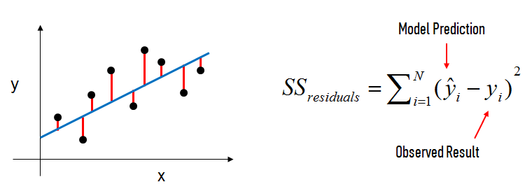
In the diagram above:
- The black dots are the observed values of x and y.
- The blue line is our least squares line.
- The red lines are the residuals, which are the vertical distances between the observed values and the least squares line.
# create X and y
n_samples = X.shape[0]
X_ = np.c_[np.ones(n_samples), X]
Lets suppose the following betas
beta_ini = np.array([-1, 1])
# h
def lr_h(beta,x):
    return np.dot(beta, x.T)
# scatter plot
plt.scatter(X, y)

# Plot the linear regression
x = np.c_[np.ones(2), [X.min(), X.max()]]
plt.plot(x[:, 1], lr_h(beta_ini, x), 'r', lw=5)
plt.xlabel('Area')
plt.ylabel('Price')
<matplotlib.text.Text at 0x7f0448eb2b38>

Lets calculate the error of such regression
# Cost function
def lr_cost_func(beta, x, y):
    # Can be vectorized
    res = 0
    for i in range(x.shape[0]):
        res += (lr_h(beta,x[i, :]) - y[i]) ** 2
    res *= 1 / (2*x.shape[0])
    return res
lr_cost_func(beta_ini, X_, y)
0.64501240712187469
Understanding the cost function
Lets see how the cost function looks like for different values of $\beta$
beta0 = np.arange(-15, 20, 1)
beta1 = 2
cost_func=[]
for beta_0 in beta0:
    cost_func.append(lr_cost_func(np.array([beta_0, beta1]), X_, y) )

plt.plot(beta0, cost_func)
plt.xlabel('beta_0')
plt.ylabel('J(beta)')
<matplotlib.text.Text at 0x7f0448ea1a90>

beta0 = 0
beta1 = np.arange(-15, 20, 1)
cost_func=[]
for beta_1 in beta1:
    cost_func.append(lr_cost_func(np.array([beta0, beta_1]), X_, y) )

plt.plot(beta1, cost_func)
plt.xlabel('beta_1')
plt.ylabel('J(beta)')
<matplotlib.text.Text at 0x7f0448e0cb38>

Analyzing both at the same time
beta0 = np.arange(-5, 7, 0.2)
beta1 = np.arange(-5, 7, 0.2)
cost_func = pd.DataFrame(index=beta0, columns=beta1)

for beta_0 in beta0:
    for beta_1 in beta1:
        cost_func.ix[beta_0, beta_1] = lr_cost_func(np.array([beta_0, beta_1]), X_, y)
betas = np.transpose([np.tile(beta0, beta1.shape[0]), np.repeat(beta1, beta0.shape[0])])
fig = plt.figure(figsize=(10, 10))
ax = fig.gca(projection='3d')
ax.plot_trisurf(betas[:, 0], betas[:, 1], cost_func.T.values.flatten(), cmap=cm.jet, linewidth=0.1)
ax.set_xlabel('beta_0')
ax.set_ylabel('beta_1')
ax.set_zlabel('J(beta)')
plt.show()

It can also be seen as a contour plot
contour_levels = [0, 0.1, 0.25, 0.5, 0.75, 1, 1.5, 2, 3, 4, 5, 7, 10, 12, 15, 20]
plt.contour(beta0, beta1, cost_func.T.values, contour_levels)
plt.xlabel('beta_0')
plt.ylabel('beta_1')
<matplotlib.text.Text at 0x7f04474f56d8>

Lets understand how different values of betas are observed on the contour plot
betas = np.array([[0, 0],
                 [-1, -1],
                 [-5, 5],
                 [3, -2]])
for beta in betas:
    print('\n\nLinear Regression with betas ', beta)
    f, (ax1, ax2) = plt.subplots(1,2, figsize=(12, 6))
    ax2.contour(beta0, beta1, cost_func.T.values, contour_levels)
    ax2.set_xlabel('beta_0')
    ax2.set_ylabel('beta_1')
    ax2.scatter(beta[0], beta[1], s=50)

    # scatter plot
    ax1.scatter(X, y)

    # Plot the linear regression
    x = np.c_[np.ones(2), [X.min(), X.max()]]
    ax1.plot(x[:, 1], lr_h(beta, x), 'r', lw=5)
    ax1.set_xlabel('Area')
    ax1.set_ylabel('Price')
    plt.show()
Linear Regression with betas [0 0]

Linear Regression with betas [-1 -1]

Linear Regression with betas [-5 5]

Linear Regression with betas [ 3 -2]

Gradient descent
Have some function $J(\beta_0, \beta_1)$
Want $\min_{\beta_0, \beta_1}J(\beta_0, \beta_1)$
Process:
Start with some $\beta_0, \beta_1$
Keep changing $\beta_0, \beta_1$ to reduce $J(\beta_0, \beta_1)$
until hopefully end up at a minimum
For the particular case of linear regression with one variable and one intercept the gradient is calculated as:
$$\frac{\partial }{\partial \beta_j} J(\beta_0, \beta_1) = \frac{\partial }{\partial \beta_j} \frac{1}{2n}\sum_{i=1}^n (h_\beta(x_i)-y_i)^2$$
$$\frac{\partial }{\partial \beta_j} J(\beta_0, \beta_1) = \frac{\partial }{\partial \beta_j} \frac{1}{2n}\sum_{i=1}^n (\beta_0 + \beta_1x_i-y_i)^2$$
$ j = 0: \frac{\partial }{\partial \beta_0} = \frac{1}{n}\sum_{i=1}^n (\beta_0 + \beta_1x_i-y_i)$
$ j = 1: \frac{\partial }{\partial \beta_1} = \frac{1}{n}\sum_{i=1}^n (\beta_0 + \beta_1x_i-y_i) \cdot x_i$
Calculate gradient
# gradient calculation
beta_ini = np.array([-1.5, 0.])

def gradient(beta, x, y):
    # Not vectorized
    gradient_0  = 1 / x.shape[0] * ((lr_h(beta, x) - y).sum())
    gradient_1  = 1 / x.shape[0] * ((lr_h(beta, x) - y)* x[:, 1]).sum()

    return np.array([gradient_0, gradient_1])

gradient(beta_ini, X_, y)
array([-1.5 , -0.85498759])
Gradient descent algorithm
def gradient_descent(x, y, beta_ini, alpha, iters):
    betas = np.zeros((iters, beta_ini.shape[0] + 1))

    beta = beta_ini
    for iter_ in range(iters):

        betas[iter_, :-1] = beta
        betas[iter_, -1] = lr_cost_func(beta, x, y)
        beta -= alpha * gradient(beta, x, y)

    return betas
iters = 100
alpha = 0.05
beta_ini = np.array([-4., -4.])

betas =  gradient_descent(X_, y, beta_ini, alpha, iters)
Lets see the evolution of the cost per iteration
plt.plot(range(iters), betas[:, -1])
plt.xlabel('iteration')
plt.ylabel('J(beta)')
<matplotlib.text.Text at 0x7f0448e1b7f0>

Understanding what it is doing in each iteration
betas_ = betas[range(0, iters, 10), :-1]
for i, beta in enumerate(betas_):
    print('\n\nLinear Regression with betas ', beta)
    f, (ax1, ax2) = plt.subplots(1,2, figsize=(12, 6))
    ax2.contour(beta0, beta1, cost_func.T.values, contour_levels)
    ax2.set_xlabel('beta_0')
    ax2.set_ylabel('beta_1')
    ax2.scatter(beta[0], beta[1], c='r', s=50)

    if i > 0:
        for beta_ in betas_[:i]:
            ax2.scatter(beta_[0], beta_[1], s=50)

    # scatter plot
    ax1.scatter(X, y)

    # Plot the linear regression
    x = np.c_[np.ones(2), [X.min(), X.max()]]
    ax1.plot(x[:, 1], lr_h(beta, x), 'r', lw=5)
    ax1.set_xlabel('Area')
    ax1.set_ylabel('Price')
    plt.show()
Linear Regression with betas [-4. -4.]

Linear Regression with betas [-2.39494776 -2.05187282]

Linear Regression with betas [-1.43394369 -0.88545711]

Linear Regression with betas [-0.85855506 -0.18708094]

Linear Regression with betas [-0.51404863 0.23106267]
Estimated Betas
betas[-1, :-1]
beta = np.dot(np.linalg.inv(np.dot(X_.T, X_)),np.dot(X_.T, y))
beta
Estimating the regression using sklearn
Using OLS
# import
from sklearn.linear_model import LinearRegression
# Initialize
linreg = LinearRegression(fit_intercept=False)
# Fit
linreg.fit(X_, y)
linreg.coef_
Using (Stochastic) Gradient Descent*
*Differs from normal gradient descent by updating the weights with each example. This converges faster for large datasets
# import
from sklearn.linear_model import SGDRegressor
# Initialize
linreg2 = SGDRegressor(fit_intercept=False, n_iter=100)
# Fit
linreg2.fit(X_, y)
linreg2.coef_
Comparing OLS and GD
| Gradient Descent | Normal Equation |
|---|---|
| Need to choose $\alpha$ | No need to choose $\alpha$ |
| Needs many iterations | Don't need to iterate |
| Works weel even when $k$ is large | Slow if $k$ is very large |
| Need to compute $(X^TX)^{-1}$ |
Linear regression with multiple variables
Lets create a new freature $ area^2 $
data['area2'] = data['area'] ** 2
data.head()
Notation review
- n = n_samples = number of examples
- k = number of features
- y = price
- $x^{(i)}$ = features of the $i$ example
i = 2
data.ix[2, ['area', 'area2']]
- $x_j^{(i)}$ = value of the $j$ feature of the $i$ example
i = 2
j = 2
data.ix[2, 'area2']
Create new matrix X and scale
X = data[['area', 'area2']].values
X[0:5]
from sklearn.preprocessing import StandardScaler
ss = StandardScaler(with_mean=True, with_std=True)
ss.fit(X.astype(np.float))
X = ss.transform(X.astype(np.float))
ss.mean_, ss.scale_
X[0:5]
X_ = np.c_[np.ones(n_samples), X]
X_[0:5]
Cost function
The goal became to estimate the parameters $\beta$ that minimize the sum of squared residuals
$$J(\beta)=\frac{1}{2n}\sum_{i=1}^n (h_\beta(x^{(i)})-y_i)^2$$
$$h_\beta(x^{(i)}) = \sum_{j=0}^k \beta_j x_j^{(i)}$$
$$J(\beta)=\frac{1}{2n}\sum_{i=1}^n \left( \left( \sum_{j=0}^k \beta_j x_j^{(i)}\right) -y_i \right)^2$$
Note that $x^0$ is refering to the column of ones
beta_ini = np.array([0., 0., 0.])

# gradient calculation
def gradient(beta, x, y):
    return 1 / x.shape[0] * np.dot((lr_h(beta, x) - y).T, x)

gradient(beta_ini, X_, y)
beta_ini = np.array([0., 0., 0.])
alpha = 0.005
iters = 100
betas = gradient_descent(X_, y, beta_ini, alpha, iters)

# Print iteration vs J
plt.plot(range(iters), betas[:, -1])
plt.xlabel('iteration')
plt.ylabel('J(beta)')
Aparently the cost function is not converging
Lets change alpha and increase the number of iterations
beta_ini = np.array([0., 0., 0.])
alpha = 0.5
iters = 1000
betas = gradient_descent(X_, y, beta_ini, alpha, iters)

# Print iteration vs J
plt.plot(range(iters), betas[:, -1])
plt.xlabel('iteration')
plt.ylabel('J(beta)')
print('betas using gradient descent\n', betas[-1, :-1])
Using the normal equations
betas_ols = np.dot(np.linalg.inv(np.dot(X_.T, X_)),np.dot(X_.T, y))
betas_ols
Difference
betas_ols - betas[-1, :-1]
x = np.array([3000., 3000.**2])

# scale
x_scaled = ss.transform(x.reshape(1, -1))
x_ = np.c_[1, x_scaled]
x_
y_pred = lr_h(betas_ols, x_)
y_pred
y_pred = y_pred * y_std + y_mean
y_pred
Using sklearn
from sklearn.linear_model import SGDRegressor
from sklearn.linear_model import LinearRegression

clf1 = LinearRegression()
clf2 = SGDRegressor(n_iter=10000)
When using sklearn there is no need to create the intercept
Also sklearn works with pandas
clf1.fit(data[['area', 'area2']], data[' price'])
clf2.fit(X, y)
Making predictions
clf1.predict(x.reshape(1, -1))
clf2.predict(x_scaled.reshape(1, -1)) * y_std + y_mean
Evaluation metrics for regression problems
Evaluation metrics for classification problems, such as accuracy, are not useful for regression problems. We need evaluation metrics designed for comparing continuous values.
Here are three common evaluation metrics for regression problems:
Mean Absolute Error (MAE) is the mean of the absolute value of the errors:
$$\frac 1n\sum_{i=1}^n|y_i-\hat{y}_i|$$Mean Squared Error (MSE) is the mean of the squared errors:
$$\frac 1n\sum_{i=1}^n(y_i-\hat{y}_i)^2$$Root Mean Squared Error (RMSE) is the square root of the mean of the squared errors:
$$\sqrt{\frac 1n\sum_{i=1}^n(y_i-\hat{y}_i)^2}$$y_pred = clf1.predict(data[['area', 'area2']])
from sklearn import metrics
import numpy as np
print('MAE:', metrics.mean_absolute_error(data[' price'], y_pred))
print('MSE:', metrics.mean_squared_error(data[' price'], y_pred))
print('RMSE:', np.sqrt(metrics.mean_squared_error(data[' price'], y_pred)))
Comparing these metrics:
- MAE is the easiest to understand, because it's the average error.
- MSE is more popular than MAE, because MSE "punishes" larger errors, which tends to be useful in the real world.
- RMSE is even more popular than MSE, because RMSE is interpretable in the "y" units.
All of these are loss functions, because we want to minimize them.
Comparing linear regression with other models
Advantages of linear regression:
- Simple to explain
- Highly interpretable
- Model training and prediction are fast
- No tuning is required (excluding regularization)
- Features don't need scaling
- Can perform well with a small number of observations
- Well-understood
Disadvantages of linear regression:
- Presumes a linear relationship between the features and the response
- Performance is (generally) not competitive with the best supervised learning methods due to high bias
- Can't automatically learn feature interactions