%matplotlib inline
import numpy as np
import pandas as pd
import random
import matplotlib.pyplot as plt
plt.style.use('ggplot')
from collections import Counter
Converting state polling average to probability
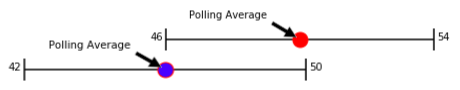
The state polling average is the average from multiple polling companies using different margins of error. For example, if a candidate has a polling average of 50% with an assumed margin of error of +/- 4, that means the truth is in the range of 46 to 54. Their opponent has a polling average of 46% with an assumed margin of error of +/- 4, that means the truth is in the range of 42 to 50.
This means we can have one candidate leading in the polls but ultimately lose the election.
 It also means we can have the candidate that lead in the polls win larger than expected.

Polling average alone does not give us the probability of a candidate winning. The candidate in the lead would win 100% of the time.
x = 50
y = 46
wins = 0 # number of wins x over y
number_of_elections = 10000
for i in range(number_of_elections):
    victory = x - y
    if victory >= 1:
        wins += 1
wins_percentage = str((float(wins) / number_of_elections)*100)+'%'
print('Candidate x wins:', wins_percentage,'of', number_of_elections,'elections')
Candidate x wins: 100.0% of 10000 elections
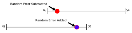
Instead, we will randomly add the margin of error to a candidate's polling average.
n = 4
random.choice(range((n*-1),(n+1),1))
3
x = 50
y = 46
n = 4
wins = 0
number_of_elections = 10000
for i in range(number_of_elections):
    moe_x = random.choice(range((n*-1),(n+1),1)) # random selection of margin or error for candidate x
    moe_y = random.choice(range((n*-1),(n+1),1)) # different margin of error for candidate y
    x1 = x + moe_x
    y1 = y + moe_y
    victory = x1 - y1
    if victory >= 1:
        wins += 1
wins_percentage = str((float(wins) / number_of_elections)*100)+'%'
print('Candidate x wins:', wins_percentage,'of', number_of_elections,'elections')
Candidate x wins: 81.58% of 10000 elections
Note that a candidate with a 4 point lead only wins 81% of the time. Keep in mind that a tie is not a victory.
What if we run it again? Will the percentage stay the same?
x = 50
y = 46
n = 4
wins = 0 # number of wins x over y
number_of_elections = 10000
for i in range(number_of_elections):
    moe_x = random.choice(range((n*-1),(n+1),1)) # random selection of margin or error for candidate x
    moe_y = random.choice(range((n*-1),(n+1),1)) # different margin of error for candidate y
    x1 = x + moe_x
    y1 = y + moe_y
    victory = x1 - y1
    if victory >= 1: # cannot be a tie
        wins += 1
wins_percentage = str((float(wins) / number_of_elections)*100)+'%'
print('Candidate x wins:', wins_percentage,'of', number_of_elections,'elections')
Candidate x wins: 81.44% of 10000 elections
It is still about 81%. Let's try doubling the number of simulated elections.
x = 50
y = 46
n = 4
wins = 0
number_of_elections = 20000 # previously we used 10,000
for i in range(number_of_elections):
    moe_x = random.choice(range((n*-1),(n+1),1))
    moe_y = random.choice(range((n*-1),(n+1),1))
    x1 = x + moe_x
    y1 = y + moe_y
    victory = x1 - y1
    if victory >= 1:
        wins += 1
wins_percentage = str((float(wins) / number_of_elections)*100)+'%'
print('Candidate x wins:', wins_percentage,'of', number_of_elections,'elections')
Candidate x wins: 81.41000000000001% of 20000 elections
x = 50
y = 46
n = 4
wins = 0
number_of_elections = 20000 # previously we used 10,000
for i in range(number_of_elections):
    moe_x = random.choice(range((n*-1),(n+1),1))
    moe_y = random.choice(range((n*-1),(n+1),1))
    x1 = x + moe_x
    y1 = y + moe_y
    victory = x1 - y1
    if victory >= 1:
        wins += 1
wins_percentage = str((float(wins) / number_of_elections)*100)+'%'
print('Candidate x wins:', wins_percentage,'of', number_of_elections,'elections')
Candidate x wins: 81.89% of 20000 elections
What about 100,000?
x = 50
y = 46
n = 4
wins = 0
number_of_elections = 100000 # previously we used 20,000
for i in range(number_of_elections):
    moe_x = random.choice(range((n*-1),(n+1),1))
    moe_y = random.choice(range((n*-1),(n+1),1))
    x1 = x + moe_x
    y1 = y + moe_y
    victory = x1 - y1
    if victory >= 1:
        wins += 1
wins_percentage = str((float(wins) / number_of_elections)*100)+'%'
print('Candidate x wins:', wins_percentage,'of', number_of_elections,'elections')
Candidate x wins: 81.286% of 100000 elections
x = 50
y = 46
n = 4
wins = 0
number_of_elections = 100000 # previously we used 20,000
for i in range(number_of_elections):
    moe_x = random.choice(range((n*-1),(n+1),1))
    moe_y = random.choice(range((n*-1),(n+1),1))
    x1 = x + moe_x
    y1 = y + moe_y
    victory = x1 - y1
    if victory >= 1:
        wins += 1
wins_percentage = str((float(wins) / number_of_elections)*100)+'%'
print('Candidate x wins:', wins_percentage,'of', number_of_elections,'elections')
Candidate x wins: 81.541% of 100000 elections
1,000,000?
x = 50
y = 46
n = 4
wins = 0
number_of_elections = 1000000 # previously we used 100,000
for i in range(number_of_elections):
    moe_x = random.choice(range((n*-1),(n+1),1))
    moe_y = random.choice(range((n*-1),(n+1),1))
    x1 = x + moe_x
    y1 = y + moe_y
    victory = x1 - y1
    if victory >= 1:
        wins += 1
wins_percentage = str((float(wins) / number_of_elections)*100)+'%'
print('Candidate x wins:', wins_percentage,'of', number_of_elections,'elections')
Candidate x wins: 81.4585% of 1000000 elections
x = 50
y = 46
n = 4
wins = 0
number_of_elections = 1000000 # previously we used 100,000
for i in range(number_of_elections):
    moe_x = random.choice(range((n*-1),(n+1),1))
    moe_y = random.choice(range((n*-1),(n+1),1))
    x1 = x + moe_x
    y1 = y + moe_y
    victory = x1 - y1
    if victory >= 1:
        wins += 1
wins_percentage = str((float(wins) / number_of_elections)*100)+'%'
print('Candidate x wins:', wins_percentage,'of', number_of_elections,'elections')
Candidate x wins: 81.5544% of 1000000 elections
We have the probability stabilizing, but do we need to do Monte Carlo simulations or can we calculate the probability to get an accurate number? Let's look at the range again.
Candidate x can end up winning 46, 47, 48, 49, 50, 51, 52, 53, or 54 votes.
Candidate y can end up winning 42, 43, 44, 45, 46, 47, 48, 49, or 50 votes.
A margin of error of 4 means both candidates have a 1 out of 9 probability (4 below average, average, 4 above).
Candidate y can only win with 47, 48, 49, or 50 (a 4 out of 9 probability) but it is dependent on candidate x.
For candidate y to win with a 47 (1 out of 9 probability), candidate y must get 46 (1 out of 9 probability).
For candidate y to win with a 48 (2 out of 9 probability), candidate y must get 47 or less (2 out of 9 probability).
For candidate y to win with a 49 (3 out of 9 probability), candidate y must get 48 or less (3 out of 9 probability).
For candidate y to win with a 50 (4 out of 9 probability), candidate y must get 49 or less (4 out of 9 probability).
We can do the complicated combinatorics or we can do a quick Monte Carlo simulation that gets us pretty close.
def moe(x, y, n):
    moe_x = random.choice(range((n*-1),(n+1),1))
    moe_y = random.choice(range((n*-1),(n+1),1))
    x += moe_x
    y += moe_y
    return x, y

def sim(x, y, n, number_of_elections=20000):
    x = int(x)
    y = int(y)
    n = int(n)
    wins = 0
    for i in range(number_of_elections):
        x1, y1 = moe(x, y, n)
        victory = x1 - y1
        if victory >= 1:
            wins += 1
    wins_percentage = str((float(wins) / number_of_elections)*100)+'%'
    return wins_percentage
Let's stick with our previous example of candidate x averaging 50 and candidate y averaging 46 with a margin of error of 4
x = 50
y = 46
n = 4
sim(x,y,n)
'81.06%'
Margin of Error
Let's take a quick look how those probabilities change as we increase the margin of error
x = 50
y = 46
n = 4
print('Candidate x winning probability with a MoE of 4:', sim(x,y,n))
n = 5
print('Candidate x winning probability with a MoE of 5:', sim(x,y,n))
n = 6
print('Candidate x winning probability with a MoE of 6:', sim(x,y,n))
n = 7
print('Candidate x winning probability with a MoE of 7:', sim(x,y,n))
n = 8
print('Candidate x winning probability with a MoE of 8:', sim(x,y,n))
n = 9
print('Candidate x winning probability with a MoE of 9:', sim(x,y,n))
n = 10
print('Candidate x winning probability with a MoE of 10:', sim(x,y,n))
Candidate x winning probability with a MoE of 4: 81.69%
Candidate x winning probability with a MoE of 5: 76.885%
Candidate x winning probability with a MoE of 6: 73.76%
Candidate x winning probability with a MoE of 7: 70.38499999999999%
Candidate x winning probability with a MoE of 8: 68.61%
Candidate x winning probability with a MoE of 9: 66.97%
Candidate x winning probability with a MoE of 10: 65.66%
We are using unweighted polling averages. This means that every poll entered into the average is treated like all others. Polling aggregators claim they weight individual polls in order to produce correct probabilities.
It is universally understood that a prediction above 50% is a prediction for that outcome. The strength of that prediction is how far above 50% that probability may be.
For example, a 99% probability is a more confident prediction than 65%.
To clarify:
Prediction is above 50%
Probability is confidence in the prediction
Applying State Probabilities to the 2016 Election
df = pd.read_csv('backtest2016.csv')
We need to decide what margin of error to use. We can take a guess or we can look at the actual results.
Let's create a margin of victory column and see what we have.
df['spread'] = abs(df['trump_rcp'] - df['clinton_rcp'])
df.plot(x='state',y='spread',kind='bar',figsize=(16,4),
        title='Polling Average Spread by State/District',legend=False)
<matplotlib.axes._subplots.AxesSubplot at 0x116182d68>

We can see from the chart above there are states that are "safe states" for candidates. These safe states are states in which one candidate does not overlap the other within the margin of error. In other words, one candidate's lowest possible result is above another candidate's highest possible result.
Let's refer to the qualitative experts to find a cutoff for what constitutes a "safe state." For this we will use the Cook Political Report.
qual = pd.read_csv('aggpreds2016.csv')
qual = qual[['State','Cook']]
rep_safe = list(qual[qual['Cook'].str.startswith('Solid R', na=False)]['State'].values)
qual[qual['Cook'].str.startswith('Solid R', na=False)]
| State | Cook | |
|---|---|---|
| 35 | Mississippi | Solid Rep. |
| 40 | Louisiana | Solid Rep. |
| 41 | Montana | Solid Rep. |
| 42 | Nebraska (CD 1)* | Solid Rep. |
| 43 | West Virginia | Solid Rep. |
| 44 | Tennessee | Solid Rep. |
| 45 | North Dakota | Solid Rep. |
| 46 | Kansas | Solid Rep. |
| 47 | Alabama | Solid Rep. |
| 48 | Arkansas | Solid Rep. |
| 49 | Nebraska | Solid Rep. |
| 50 | South Dakota | Solid Rep. |
| 51 | Idaho | Solid Rep. |
| 52 | Kentucky | Solid Rep. |
| 53 | Oklahoma | Solid Rep. |
| 54 | Wyoming | Solid Rep. |
| 55 | Nebraska (CD 3)* | Solid Rep. |
dem_safe = list(qual[qual['Cook'].str.startswith('Solid D', na=False)]['State'].values)
qual[qual['Cook'].str.startswith('Solid D', na=False)]
| State | Cook | |
|---|---|---|
| 0 | D.C. | Solid Dem. |
| 1 | California | Solid Dem. |
| 2 | Maryland | Solid Dem. |
| 3 | Hawaii | Solid Dem. |
| 4 | Vermont | Solid Dem. |
| 5 | New York | Solid Dem. |
| 6 | Rhode Island | Solid Dem. |
| 7 | Illinois | Solid Dem. |
| 8 | Washington | Solid Dem. |
| 9 | New Jersey | Solid Dem. |
| 10 | Connecticut | Solid Dem. |
| 11 | Maine (CD 1)* | Solid Dem. |
| 12 | Delaware | Solid Dem. |
| 13 | Massachusetts | Solid Dem. |
| 14 | Oregon | Solid Dem. |
spread_states = df[df['spread'] >= 12]['state'].values
df[df['spread'] >= 12]['state']
17             Connecticut
22                   Texas
26            South Dakota
27               Tennessee
28                  Alaska
29                  Kansas
33              Washington
34            Rhode Island
35                Delaware
36           Massachusetts
37                New York
38              California
39    District Of Columbia
40                  Hawaii
41                Maryland
42                 Vermont
43               Louisiana
44             Mississippi
45                 Alabama
46                Arkansas
47                Kentucky
48                   Idaho
49                Nebraska
50            North Dakota
51                Oklahoma
52           West Virginia
53                 Wyoming
Name: state, dtype: object
for state in spread_states:
    if state in rep_safe or state in dem_safe:
        pass
    else:
        print(state)
Texas
Alaska
District Of Columbia
If we use 6 as our margin of error, we can have all the states above 12 land in the "safe state" category which will be represented by a probability of 100% for the safe candidate and 0% for the opponent.
trump_x = df['trump_rcp'].values
clinton_y = df['clinton_rcp'].values

clinton_x = df['clinton_rcp'].values
trump_y = df['trump_rcp'].values
def sim(x, y, n, number_of_elections=20000):
    x = int(x)
    y = int(y)
    n = int(n)
    wins = 0
    for i in range(number_of_elections):
        x1, y1 = moe(x, y, n)
        victory = x1 - y1
        if victory >= 1:
            wins += 1
    wins_percentage = float(wins) / number_of_elections
    return wins_percentage
trump_rcp_prob = []
for x, y in zip(trump_x, clinton_y):
    nwp = sim(x,y,6)
    trump_rcp_prob.append(100*nwp)

clinton_rcp_prob = []
for x, y in zip(clinton_x, trump_y):
    nwp = sim(x,y,6)
    clinton_rcp_prob.append(100*nwp)

df['trump_rcp_prob'] = trump_rcp_prob
df['clinton_rcp_prob'] = clinton_rcp_prob
df.head()
| state | ec | clinton_rcp | trump_rcp | clinton_actual | trump_actual | spread | trump_rcp_prob | clinton_rcp_prob | |
|---|---|---|---|---|---|---|---|---|---|
| 0 | Florida | 29 | 46.4 | 46.6 | 47.80 | 49.02 | 0.2 | 45.405 | 46.535 |
| 1 | Ohio | 18 | 42.3 | 45.8 | 43.56 | 51.69 | 3.5 | 67.455 | 27.085 |
| 2 | Michigan | 16 | 45.4 | 42.0 | 47.27 | 47.50 | 3.4 | 26.580 | 67.155 |
| 3 | Pennsylvania | 20 | 46.2 | 44.3 | 47.46 | 48.18 | 1.9 | 32.550 | 60.570 |
| 4 | New Hampshire | 4 | 43.3 | 42.7 | 46.98 | 46.61 | 0.6 | 38.760 | 54.105 |
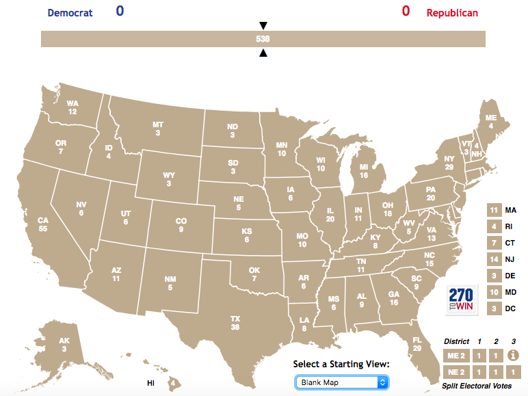
The Electoral College
Now that we have probabilities assigned to the states and districts, we can bring in the Electoral College scoring system.
For more detail on how it works, you can read about it here
print('Maximum electoral college votes possible:', np.sum(df['ec']))
print('Minimum electoral college votes to win:', int((np.sum(df['ec'])/2) + 1) )
Maximum electoral college votes possible: 538
Minimum electoral college votes to win: 270
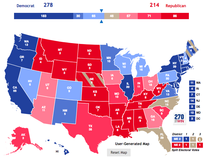
Let's see which of the two candidates are in the lead according to our probabilities
print('Trump Most Likely Electoral College Results::', np.sum(df['ec'][df['trump_rcp_prob'] >= 50]))
print()
print('Clinton Most Likely Electoral College Results::', np.sum(df['ec'][df['clinton_rcp_prob'] >= 50]))
Trump Most Likely Electoral College Results:: 230

Clinton Most Likely Electoral College Results:: 272
print('538 - (272+230):',538 - (272+230) )
538 - (272+230): 36
Which states are missing?
unc_states = list(df[ (df['trump_rcp_prob'] <= 50) & (df['clinton_rcp_prob'] <= 50) ]['state'].values)
df[ (df['trump_rcp_prob'] <= 50) & (df['clinton_rcp_prob'] <= 50) ][['state','ec']]
| state | ec | |
|---|---|---|
| 0 | Florida | 29 |
| 5 | Maine CD2 | 1 |
| 11 | Nevada | 6 |
This is another reason why the 2016 Presidential Election was unique. We have two states and a district where neither major candidate had a 50% probability of winning. These are statistically "tossup states" since we can assign a probability but not a prediction.
Reusing our Simulation to Create Election Winning Probabilities
Before we can simulate the electoral college results, we need to address something unique with our probability assignments. A state awarding its electoral college votes to a candidate should be 100%, yet we have a number of states and districts that do not total 100%.
Let us determine this probability for each state and make that our uncertainty probability.
df['unc_prob'] = 100 - (df['trump_rcp_prob'] + df['clinton_rcp_prob'])
df[['state','trump_rcp_prob','clinton_rcp_prob','unc_prob']].sort_values('unc_prob',ascending=False)
| state | trump_rcp_prob | clinton_rcp_prob | unc_prob | |
|---|---|---|---|---|
| 5 | Maine CD2 | 45.725 | 45.765 | 8.510 |
| 11 | Nevada | 45.750 | 46.185 | 8.065 |
| 0 | Florida | 45.405 | 46.535 | 8.060 |
| 7 | North Carolina | 53.770 | 38.810 | 7.420 |
| 4 | New Hampshire | 38.760 | 54.105 | 7.135 |
| 3 | Pennsylvania | 32.550 | 60.570 | 6.880 |
| 2 | Michigan | 26.580 | 67.155 | 6.265 |
| 14 | Iowa | 66.950 | 27.065 | 5.985 |
| 1 | Ohio | 67.455 | 27.085 | 5.460 |
| 10 | Colorado | 27.095 | 67.465 | 5.440 |
| 12 | New Mexico | 16.675 | 77.945 | 5.380 |
| 13 | Arizona | 73.075 | 21.635 | 5.290 |
| 20 | South Carolina | 73.425 | 21.455 | 5.120 |
| 9 | Georgia | 78.895 | 16.775 | 4.330 |
| 8 | Virginia | 17.085 | 78.630 | 4.285 |
| 6 | Maine | 16.980 | 78.870 | 4.150 |
| 15 | Wisconsin | 12.480 | 83.590 | 3.930 |
| 16 | Oregon | 6.175 | 91.270 | 2.555 |
| 30 | Nebraska CD2 | 94.120 | 3.395 | 2.485 |
| 19 | Maine CD1 | 3.415 | 94.335 | 2.250 |
| 18 | Minnesota | 1.785 | 96.220 | 1.995 |
| 24 | Utah | 96.400 | 1.715 | 1.885 |
| 25 | Montana | 96.440 | 1.690 | 1.870 |
| 21 | Indiana | 98.215 | 0.535 | 1.250 |
| 23 | Missouri | 98.270 | 0.510 | 1.220 |
| 32 | New Jersey | 0.535 | 98.295 | 1.170 |
| 27 | Tennessee | 99.400 | 0.000 | 0.600 |
| 31 | Illinois | 0.000 | 99.410 | 0.590 |
| 22 | Texas | 99.485 | 0.000 | 0.515 |
| 26 | South Dakota | 100.000 | 0.000 | 0.000 |
| 42 | Vermont | 0.000 | 100.000 | 0.000 |
| 52 | West Virginia | 100.000 | 0.000 | 0.000 |
| 51 | Oklahoma | 100.000 | 0.000 | 0.000 |
| 50 | North Dakota | 100.000 | 0.000 | 0.000 |
| 49 | Nebraska | 100.000 | 0.000 | 0.000 |
| 48 | Idaho | 100.000 | 0.000 | 0.000 |
| 47 | Kentucky | 100.000 | 0.000 | 0.000 |
| 46 | Arkansas | 100.000 | 0.000 | 0.000 |
| 45 | Alabama | 100.000 | 0.000 | 0.000 |
| 44 | Mississippi | 100.000 | 0.000 | 0.000 |
| 43 | Louisiana | 100.000 | 0.000 | 0.000 |
| 40 | Hawaii | 0.000 | 100.000 | 0.000 |
| 41 | Maryland | 0.000 | 100.000 | 0.000 |
| 28 | Alaska | 100.000 | 0.000 | 0.000 |
| 39 | District Of Columbia | 0.000 | 100.000 | 0.000 |
| 38 | California | 0.000 | 100.000 | 0.000 |
| 37 | New York | 0.000 | 100.000 | 0.000 |
| 36 | Massachusetts | 0.000 | 100.000 | 0.000 |
| 35 | Delaware | 0.000 | 100.000 | 0.000 |
| 34 | Rhode Island | 0.000 | 100.000 | 0.000 |
| 33 | Washington | 0.000 | 100.000 | 0.000 |
| 17 | Connecticut | 0.000 | 100.000 | 0.000 |
| 29 | Kansas | 100.000 | 0.000 | 0.000 |
| 53 | Wyoming | 100.000 | 0.000 | 0.000 |
Simulating One Election
ec = list(df.ec.values)
states = list(df.state.values)
cand = list(df['trump_rcp_prob'].values)
sim_election = np.random.uniform()*100
ec_total = 0
for x, y, z in zip(cand, states, ec):
    if x > sim_election:
        print('Won',y,'for',z,'electoral college votes')
        ec_total += z
print()
print('Final Results:',ec_total,'electoral college votes')
Won Indiana for 11 electoral college votes
Won Texas for 38 electoral college votes
Won Missouri for 10 electoral college votes
Won Utah for 6 electoral college votes
Won Montana for 3 electoral college votes
Won South Dakota for 3 electoral college votes
Won Tennessee for 11 electoral college votes
Won Alaska for 3 electoral college votes
Won Kansas for 6 electoral college votes
Won Nebraska CD2 for 1 electoral college votes
Won Louisiana for 8 electoral college votes
Won Mississippi for 6 electoral college votes
Won Alabama for 9 electoral college votes
Won Arkansas for 6 electoral college votes
Won Kentucky for 8 electoral college votes
Won Idaho for 4 electoral college votes
Won Nebraska for 4 electoral college votes
Won North Dakota for 3 electoral college votes
Won Oklahoma for 7 electoral college votes
Won West Virginia for 5 electoral college votes
Won Wyoming for 3 electoral college votes

Final Results: 155 electoral college votes
Making state-by-state outcomes just a bit more realistic
The challenge that comes with simulations is that if it is statistically possible then it will likely show up in the simulation. Whether to leave the possibility open ultimately becomes a matter of judgement. For this simulation, we will make any state above a 5% probability eligible for a candidate to win in the simulation. This is inline with out "safe state" assessments from the qualitative experts.
ec = list(df.ec.values)
states = list(df.state.values)
cand = list(df['trump_rcp_prob'].values)
sim_election = np.random.uniform(low=0.05)*100
ec_total = 0
for x, y, z in zip(cand, states, ec):
    if x > sim_election:
        print('Won',y,'for',z,'electoral college votes')
        ec_total += z
print()
print('Final Results:',ec_total,'electoral college votes')
Won Florida for 29 electoral college votes
Won Ohio for 18 electoral college votes
Won Michigan for 16 electoral college votes
Won Pennsylvania for 20 electoral college votes
Won New Hampshire for 4 electoral college votes
Won Maine CD2 for 1 electoral college votes
Won North Carolina for 15 electoral college votes
Won Georgia for 16 electoral college votes
Won Colorado for 9 electoral college votes
Won Nevada for 6 electoral college votes
Won Arizona for 11 electoral college votes
Won Iowa for 6 electoral college votes
Won South Carolina for 9 electoral college votes
Won Indiana for 11 electoral college votes
Won Texas for 38 electoral college votes
Won Missouri for 10 electoral college votes
Won Utah for 6 electoral college votes
Won Montana for 3 electoral college votes
Won South Dakota for 3 electoral college votes
Won Tennessee for 11 electoral college votes
Won Alaska for 3 electoral college votes
Won Kansas for 6 electoral college votes
Won Nebraska CD2 for 1 electoral college votes
Won Louisiana for 8 electoral college votes
Won Mississippi for 6 electoral college votes
Won Alabama for 9 electoral college votes
Won Arkansas for 6 electoral college votes
Won Kentucky for 8 electoral college votes
Won Idaho for 4 electoral college votes
Won Nebraska for 4 electoral college votes
Won North Dakota for 3 electoral college votes
Won Oklahoma for 7 electoral college votes
Won West Virginia for 5 electoral college votes
Won Wyoming for 3 electoral college votes

Final Results: 315 electoral college votes
ec = list(df.ec.values)
states = list(df.state.values)
cand = list(df['clinton_rcp_prob'].values)
sim_election = np.random.uniform(low=0.05)*100
ec_total = 0
for x, y, z in zip(cand, states, ec):
    if x > sim_election:
        print('Won',y,'for',z,'electoral college votes')
        ec_total += z
print()
print('Final Results:',ec_total,'electoral college votes')
Won Michigan for 16 electoral college votes
Won Pennsylvania for 20 electoral college votes
Won New Hampshire for 4 electoral college votes
Won Maine for 2 electoral college votes
Won Virginia for 13 electoral college votes
Won Colorado for 9 electoral college votes
Won New Mexico for 5 electoral college votes
Won Wisconsin for 10 electoral college votes
Won Oregon for 7 electoral college votes
Won Connecticut for 7 electoral college votes
Won Minnesota for 10 electoral college votes
Won Maine CD1 for 1 electoral college votes
Won Illinois for 20 electoral college votes
Won New Jersey for 14 electoral college votes
Won Washington for 12 electoral college votes
Won Rhode Island for 4 electoral college votes
Won Delaware for 3 electoral college votes
Won Massachusetts for 11 electoral college votes
Won New York for 29 electoral college votes
Won California for 55 electoral college votes
Won District Of Columbia for 3 electoral college votes
Won Hawaii for 4 electoral college votes
Won Maryland for 10 electoral college votes
Won Vermont for 3 electoral college votes

Final Results: 272 electoral college votes
Swing States
We will go back to the qualitative experts in order to determine swing states.
qual[qual['Cook'].str.startswith('Lea', na=False)]
| State | Cook | |
|---|---|---|
| 17 | Michigan | Lean Dem. |
| 19 | Wisconsin | Lean Dem. |
| 21 | Pennsylvania | Lean Dem. |
| 22 | Colorado | Lean Dem. |
| 23 | New Hampshire | Lean Dem. |
| 24 | Nevada | Lean Dem. |
| 27 | Ohio | Lean Rep. |
| 28 | Iowa | Lean Rep. |
| 30 | Utah | Lean Rep. |
| 33 | Georgia | Lean Rep. |
| 34 | Arizona | Lean Rep. |
qual[qual['Cook'].str.startswith('Tos', na=False)]
| State | Cook | |
|---|---|---|
| 25 | Florida | Tossup |
| 26 | North Carolina | Tossup |
| 29 | Maine (CD 2)* | Tossup |
| 31 | Nebraska (CD 2)* | Tossup |
We now have 13 swing states and two swing districts. The four toss ups will get their own simulation results independent of each other. For the remaining swing states, we can either group according to the qualitative experts or group according to the qualitative experts and geography. Combining the qualitative experts with state geography allows us to capture regional attitudes, interests, and opinions. For example, Utah and Arizona have different public opinion polling than Colorado and Nevada on the issue of legalized marijuana.
swing_states = ['Michigan', 'Wisconsin', 'Pennsylvania', 'Colorado', 'New Hampshire',
 'Nevada', 'Ohio', 'Iowa', 'Utah', 'Georgia', 'Arizona','Florida', 'North Carolina','Maine CD2','Nebraska CD2']
lean_r_west = ['Utah','Arizona']
lean_d_west = ['Colorado','Nevada']
lean_r_lakes = ['Ohio', 'Iowa']
lean_d_lakes = ['Michigan', 'Wisconsin', 'Pennsylvania',]
tossups = ['Florida', 'North Carolina','Maine CD2','Nebraska CD2']
ec = list(df.ec.values)
states = list(df.state.values)
cand = list(df['clinton_rcp_prob'].values)
sim_election = np.random.uniform(low=0.05)*100
lean_r_west_sim = np.random.uniform()*100
lean_d_west_sim = np.random.uniform()*100
lean_r_lakes_sim = np.random.uniform()*100
lean_d_lakes_sim = np.random.uniform()*100
ec_total = 0
for x, y, z in zip(cand, states, ec):
    if y in swing_states:
        if y in lean_r_west:
            sim_election = lean_r_west_sim
        if y in lean_d_west:
            sim_election = lean_d_west_sim
        if y in lean_r_lakes:
            sim_election = lean_r_lakes_sim
        if y in lean_d_lakes:
            sim_election = lean_d_lakes_sim
        if y in tossups:
            sim_election = np.random.uniform()*100
    if x > sim_election:
        print('Won',y,'for',z,'electoral college votes')
        ec_total += z
print()
print('Final Results:',ec_total,'electoral college votes')
Won Florida for 29 electoral college votes
Won Maine for 2 electoral college votes
Won Virginia for 13 electoral college votes
Won Colorado for 9 electoral college votes
Won Nevada for 6 electoral college votes
Won New Mexico for 5 electoral college votes
Won Wisconsin for 10 electoral college votes
Won Oregon for 7 electoral college votes
Won Connecticut for 7 electoral college votes
Won Minnesota for 10 electoral college votes
Won Maine CD1 for 1 electoral college votes
Won Illinois for 20 electoral college votes
Won New Jersey for 14 electoral college votes
Won Washington for 12 electoral college votes
Won Rhode Island for 4 electoral college votes
Won Delaware for 3 electoral college votes
Won Massachusetts for 11 electoral college votes
Won New York for 29 electoral college votes
Won California for 55 electoral college votes
Won District Of Columbia for 3 electoral college votes
Won Hawaii for 4 electoral college votes
Won Maryland for 10 electoral college votes
Won Vermont for 3 electoral college votes

Final Results: 267 electoral college votes
ec = list(df.ec.values)
states = list(df.state.values)
cand = list(df['trump_rcp_prob'].values)
ec_total = 0


sim_election = np.random.uniform(low=0.05)*100
lean_r_west_sim = np.random.uniform()*100
lean_d_west_sim = np.random.uniform()*100
lean_r_lakes_sim = np.random.uniform()*100
lean_d_lakes_sim = np.random.uniform()*100
for x, y, z in zip(cand, states, ec):
    if y in swing_states:
        if y in lean_r_west:
            sim_election = lean_r_west_sim
        if y in lean_d_west:
            sim_election = lean_d_west_sim
        if y in lean_r_lakes:
            sim_election = lean_r_lakes_sim
        if y in lean_d_lakes:
            sim_election = lean_d_lakes_sim
        if y in tossups:
            sim_election = np.random.uniform()*100
    if x > sim_election:
        print('Won',y,'for',z,'electoral college votes')
        ec_total += z
print()
print('Final Results:',ec_total,'electoral college votes')
Won Florida for 29 electoral college votes
Won Michigan for 16 electoral college votes
Won Pennsylvania for 20 electoral college votes
Won New Hampshire for 4 electoral college votes
Won Arizona for 11 electoral college votes
Won Wisconsin for 10 electoral college votes
Won South Carolina for 9 electoral college votes
Won Indiana for 11 electoral college votes
Won Texas for 38 electoral college votes
Won Missouri for 10 electoral college votes
Won Utah for 6 electoral college votes
Won Montana for 3 electoral college votes
Won South Dakota for 3 electoral college votes
Won Tennessee for 11 electoral college votes
Won Alaska for 3 electoral college votes
Won Kansas for 6 electoral college votes
Won Nebraska CD2 for 1 electoral college votes
Won Louisiana for 8 electoral college votes
Won Mississippi for 6 electoral college votes
Won Alabama for 9 electoral college votes
Won Arkansas for 6 electoral college votes
Won Kentucky for 8 electoral college votes
Won Idaho for 4 electoral college votes
Won Nebraska for 4 electoral college votes
Won North Dakota for 3 electoral college votes
Won Oklahoma for 7 electoral college votes
Won West Virginia for 5 electoral college votes
Won Wyoming for 3 electoral college votes

Final Results: 254 electoral college votes
Running 20,000 Simulations
def electoral_college(ec, cand, state, sims=10):
    cand_wins = 0
    cand_ec_total = []
    cand_states = []
    for i in range(sims):
        cand_ec = 0
        cand_state = []
        sim_election = np.random.uniform(low=0.05)*100
        lean_r_west_sim = np.random.uniform()*100
        lean_d_west_sim = np.random.uniform()*100
        lean_r_lakes_sim = np.random.uniform()*100
        lean_d_lakes_sim = np.random.uniform()*100
        for x, y, z in zip(cand, states, ec):
            if y in swing_states:
                if y in lean_r_west:
                    sim_election = lean_r_west_sim
                if y in lean_d_west:
                    sim_election = lean_d_west_sim
                if y in lean_r_lakes:
                    sim_election = lean_r_lakes_sim
                if y in lean_d_lakes:
                    sim_election = lean_d_lakes_sim
                if y in tossups:
                    sim_election = np.random.uniform()*100
            if x > sim_election:
                cand_ec += z
                cand_state.append(y)
        cand_ec_total.append(cand_ec)
        cand_states.append(cand_state)
        if cand_ec > 269:
            cand_wins += 1
    return cand_wins, cand_ec_total, cand_states
print("Monte Carlo Simulation of Electoral College Results")
print()
sims = 20000
ec = list(df.ec.values)
states = list(df.state.values)
cand_1 = list(df['clinton_rcp_prob'].values)
cand_1_wins, cand_1_ec_totals, cand_1_states = electoral_college(ec, cand_1, states, sims=sims)
print('Clinton Win Prob:', (cand_1_wins/sims)*100)
for i,j in Counter(cand_1_ec_totals).most_common(n=1):
    print('Electoral College Results: Clinton',i)
    print('Sim Percent Outcome:',j/20000)
print()
cand_2 = list(df['trump_rcp_prob'].values)
cand_2_wins, cand_2_ec_totals, cand_2_states = electoral_college(ec, cand_2, states, sims=sims)
print('Trump Win Prob:', (cand_2_wins/sims)*100)
for i,j in Counter(cand_2_ec_totals).most_common(n=1):
    print('Electoral College Results: Trump',i)
    print('Sim Percent Outcome:',j/20000)
Monte Carlo Simulation of Electoral College Results

Clinton Win Prob: 65.945
Electoral College Results: Clinton 279
Sim Percent Outcome: 0.0198

Trump Win Prob: 22.335
Electoral College Results: Trump 235
Sim Percent Outcome: 0.01955
Top 5 Results for Each Candidate
for i,j in Counter(cand_1_ec_totals).most_common(n=5):
    print('Electoral College Results: Clinton',i)
    print('Sim Percent Outcome:',j/20000)
Electoral College Results: Clinton 279
Sim Percent Outcome: 0.0198
Electoral College Results: Clinton 303
Sim Percent Outcome: 0.01715
Electoral College Results: Clinton 288
Sim Percent Outcome: 0.01685
Electoral College Results: Clinton 294
Sim Percent Outcome: 0.01485
Electoral College Results: Clinton 287
Sim Percent Outcome: 0.0143
for i,j in Counter(cand_2_ec_totals).most_common(n=5):
    print('Electoral College Results: Trump',i)
    print('Sim Percent Outcome:',j/20000)
Electoral College Results: Trump 235
Sim Percent Outcome: 0.01955
Electoral College Results: Trump 259
Sim Percent Outcome: 0.01855
Electoral College Results: Trump 250
Sim Percent Outcome: 0.0175
Electoral College Results: Trump 230
Sim Percent Outcome: 0.0165
Electoral College Results: Trump 219
Sim Percent Outcome: 0.0163
plt.figure(figsize=(18,8))
plt.hist(cand_2_ec_totals,500)
plt.hist(cand_1_ec_totals,500)
plt.axvline(x=270, color='k', linestyle='dashed')
plt.title('Simulation Results')
plt.show()

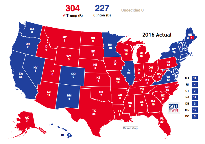
Actual 2016 Electoral College Results
Conclusion
The simulation gives us more reasonable probabilities for each candidate but does not overcorrect to replicate the 2016 Electoral College results. The polling errors in Wisconsin, Pennsylvania, and Michigan would have to have been identified prior to running simulations when assigning probabilities to each state.