Classification of Italian Wines¶

alt text

In this notebook we will be using supervised learning to classify Italian wines. The question is: Can we teach a machine to figure out which type of wine an obseration belongs to?

We will work with a famous but small dataset that can be found here (along more informaion). The data is clean, contains only numerical and no missing values. We will not do any EDA but only focus on prediction. The only preprocessing step will be standardization of the physiochemical variables.

We will be using Pandas and Scikit-Learn which are both parts of the Anaconda distribution.

In [42]:

# Download the dateset using WGET.
# If this is not possible, then just paste the URL in your browser and download 
# the file, or if you use GithubDesktop then it should be in the folder
# after a pull.


!wget https://cdn.rawgit.com/SDS-AAU/M1-2018/182abaa2/data/wine.csv

Redirecting output to ‘wget-log.1’.

In [0]:

# Importing the libraries

import numpy as np # for working with arrays
np.set_printoptions(suppress=True) # not a must but nice to avoid scientific notation


import pandas as pd # as usual for handling dataframes
pd.options.display.float_format = '{:.4f}'.format #same for pandas to turn off scientific notation

In [0]:

# Importing the dataset
dataset = pd.read_csv('wine.csv')

In [45]:

# Quick check of the dataframe proportions
dataset.shape

Out[45]:

(178, 15)

In [46]:

# Checking the first 5 rows to get familiar with the data
dataset.head()

Out[46]:

	class_label	class_name	alcohol	malic_acid	ash	alcalinity_of_ash	magnesium	total_phenols	flavanoids	nonflavanoid_phenols	proanthocyanins	color_intensity	hue	od280	proline
0	1	Barolo	14.2300	1.7100	2.4300	15.6000	127	2.8000	3.0600	0.2800	2.2900	5.6400	1.0400	3.9200	1065
1	1	Barolo	13.2000	1.7800	2.1400	11.2000	100	2.6500	2.7600	0.2600	1.2800	4.3800	1.0500	3.4000	1050
2	1	Barolo	13.1600	2.3600	2.6700	18.6000	101	2.8000	3.2400	0.3000	2.8100	5.6800	1.0300	3.1700	1185
3	1	Barolo	14.3700	1.9500	2.5000	16.8000	113	3.8500	3.4900	0.2400	2.1800	7.8000	0.8600	3.4500	1480
4	1	Barolo	13.2400	2.5900	2.8700	21.0000	118	2.8000	2.6900	0.3900	1.8200	4.3200	1.0400	2.9300	735

In [47]:

# Getting basic descriptives for all nummerical variables
dataset.describe()

Out[47]:

	class_label	alcohol	malic_acid	ash	alcalinity_of_ash	magnesium	total_phenols	flavanoids	nonflavanoid_phenols	proanthocyanins	color_intensity	hue	od280	proline
count	178.0000	178.0000	178.0000	178.0000	178.0000	178.0000	178.0000	178.0000	178.0000	178.0000	178.0000	178.0000	178.0000	178.0000
mean	1.9382	13.0006	2.3363	2.3665	19.4949	99.7416	2.2951	2.0293	0.3619	1.5909	5.0581	0.9574	2.6117	746.8933
std	0.7750	0.8118	1.1171	0.2743	3.3396	14.2825	0.6259	0.9989	0.1245	0.5724	2.3183	0.2286	0.7100	314.9075
min	1.0000	11.0300	0.7400	1.3600	10.6000	70.0000	0.9800	0.3400	0.1300	0.4100	1.2800	0.4800	1.2700	278.0000
25%	1.0000	12.3625	1.6025	2.2100	17.2000	88.0000	1.7425	1.2050	0.2700	1.2500	3.2200	0.7825	1.9375	500.5000
50%	2.0000	13.0500	1.8650	2.3600	19.5000	98.0000	2.3550	2.1350	0.3400	1.5550	4.6900	0.9650	2.7800	673.5000
75%	3.0000	13.6775	3.0825	2.5575	21.5000	107.0000	2.8000	2.8750	0.4375	1.9500	6.2000	1.1200	3.1700	985.0000
max	3.0000	14.8300	5.8000	3.2300	30.0000	162.0000	3.8800	5.0800	0.6600	3.5800	13.0000	1.7100	4.0000	1680.0000

We can see here that means and spread (standard deviation) of the features is very different and thus we will need to standardize the dataset.

"As a rule of thumb I’d say: When in doubt, just standardize the data, it shouldn’t hurt."" Sebastian Raschka

In [0]:

# Selecting the relevant data
# using the iloc selector allows to grab a range 2-15 of columns
# withouth having to call their names. That's practical
# Also, we ask for values only, as we are going to pass the data into
# the ML algorithms in the form of arrays rather than pandas DFs

X = dataset.iloc[:, 2:15].values
y = dataset.iloc[:, 1].values

Yes, there is a class_lable in the dataset but for the sake of learning and because it is very simple, we are going to construct our class_lables on our own. For this we will use the LabelEncoder from Scikit-Learn. Note that in contrast to Pandas, the Scikit-Learn is more of a (HUGE!!!) Library where you have to import different functionalities separately. You can find an index of all classes here.

In [0]:

# Encoding categorical data
from sklearn.preprocessing import LabelEncoder

Classes such as the LabelEncoder or any modely type that you import have several parameters that can (but don't have to be) specified. Also, you are usually fitting them to some data first before performind transformations. Thus, they are cutom-made for each use case and therefore you will need to define an encoder object from the imported class. This is a general philosophy behind all Scikit-Learn classes. The good news: The syntax is the same across all classes.

Below we first define a labelencoder_y and then use the fit_transform method (we could also first use fit and then transform) to turn our wine-type names into numbers.

In [0]:

# From labels to numbers
labelencoder_y = LabelEncoder()
y = labelencoder_y.fit_transform(y)

As you have seen from the descriptives above our variables lie on very different scales. Therefore, we will standardize them before going further. The procedure using the StandardScaleris exactly the same as before with the label encoder.

This scaling will for each value substract the mean (of the column) and devide it by the standard deviation, thus bringing them all on the same scale with a mean of 0 and a standard deviation of 1.

In [0]:

# Feature scaling
from sklearn.preprocessing import StandardScaler

scaler = StandardScaler()

X = scaler.fit_transform(X)

In [56]:

# We can check our transform data using pandas describe
pd.DataFrame(X).describe()

Out[56]:

	0	1	2	3	4	5	6	7	8	9	10	11	12
count	178.0000	178.0000	178.0000	178.0000	178.0000	178.0000	178.0000	178.0000	178.0000	178.0000	178.0000	178.0000	178.0000
mean	-0.0000	-0.0000	-0.0000	-0.0000	-0.0000	0.0000	-0.0000	0.0000	-0.0000	0.0000	0.0000	0.0000	-0.0000
std	1.0028	1.0028	1.0028	1.0028	1.0028	1.0028	1.0028	1.0028	1.0028	1.0028	1.0028	1.0028	1.0028
min	-2.4342	-1.4330	-3.6792	-2.6710	-2.0883	-2.1072	-1.6960	-1.8682	-2.0690	-1.6343	-2.0947	-1.8951	-1.4932
25%	-0.7882	-0.6587	-0.5721	-0.6891	-0.8244	-0.8855	-0.8275	-0.7401	-0.5973	-0.7951	-0.7676	-0.9522	-0.7846
50%	0.0610	-0.4231	-0.0238	0.0015	-0.1223	0.0960	0.1061	-0.1761	-0.0629	-0.1592	0.0331	0.2377	-0.2337
75%	0.8361	0.6698	0.6981	0.6021	0.5096	0.8090	0.8491	0.6095	0.6292	0.4940	0.7132	0.7886	0.7582
max	2.2598	3.1092	3.1563	3.1545	4.3714	2.5395	3.0628	2.4024	3.4851	3.4354	3.3017	1.9609	2.9715

In the next step we split the data into a training and a test-set. Very often you will see a split of 80/20 %

alt text

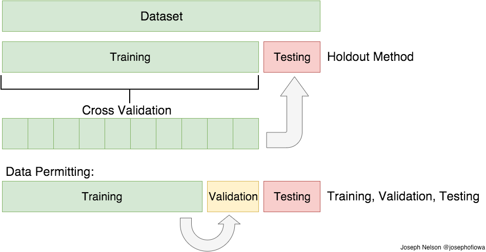
80% of the data will be used to fit a model, while we will keep 20% of the data for testing the models performance.

The train_test_split class takes 4 parameters: (X, y, test_size = 0.2, random_state = 21)

Input matrix: X
Output matrix: y
The test size: We take 20%
A random state (optional): Some number for the random generator that will shuffle the values*

*The whole random state thing is mostly for easier reproducibility and can also be let our.

In [0]:

# Splitting the dataset into the Training set and Test set

from sklearn.model_selection import train_test_split

X_train, X_test, y_train, y_test = train_test_split(X, y, test_size = 0.2, random_state = 21)

alt text

Now it's time for the model to meet the wine data.

We will be using 3 different models. The reason why we use 3 models is because, it is nice to see how easy it is to switch them aroun to experiment what works best. Since we can calculate an (kind of) objective quality measure, it is easy to compare and evaluate them agains each other.

Logistic Regression
Suport Vector Classifier
Random Forest Classifier

Remember that this is a classification problem rather than a regression. The models will be estimating probabilities for some class vs. other classes.

In [57]:

# We first import and train a Logistic Regression

from sklearn.linear_model import LogisticRegression

classifier = LogisticRegression(random_state = 22)

classifier.fit(X_train, y_train)

# After training the model we should jump further down (over the next 2 models)
# To evaluate the results

Out[57]:

LogisticRegression(C=1.0, class_weight=None, dual=False, fit_intercept=True,
          intercept_scaling=1, max_iter=100, multi_class='ovr', n_jobs=1,
          penalty='l2', random_state=22, solver='liblinear', tol=0.0001,
          verbose=0, warm_start=False)

In [59]:

# Fitting Random Forest Classification to the Training set
from sklearn.ensemble import RandomForestClassifier

classifier = RandomForestClassifier(n_estimators = 50, criterion = 'entropy', random_state = 22)

classifier.fit(X_train, y_train)

Out[59]:

RandomForestClassifier(bootstrap=True, class_weight=None, criterion='entropy',
            max_depth=None, max_features='auto', max_leaf_nodes=None,
            min_impurity_decrease=0.0, min_impurity_split=None,
            min_samples_leaf=1, min_samples_split=2,
            min_weight_fraction_leaf=0.0, n_estimators=50, n_jobs=1,
            oob_score=False, random_state=22, verbose=0, warm_start=False)

In [61]:

# Finally we train a Support Vector Classifier
from sklearn.svm import SVC

classifier = SVC(kernel = 'linear', random_state = 21)

classifier.fit(X_train, y_train)

Out[61]:

SVC(C=1.0, cache_size=200, class_weight=None, coef0=0.0,
  decision_function_shape='ovr', degree=3, gamma='auto', kernel='linear',
  max_iter=-1, probability=False, random_state=21, shrinking=True,
  tol=0.001, verbose=False)

Perhaps this time the algorithm was just lucky because of a random allocation of the data in the train-test split. To make sure which model is the most accurate, we can run a k-Fold Cross Validation deviding x_train into (here) 10 parts, training on 9 and testing on 1. This will be done 10 times, every time measuring the accuracy and finally returning the average accuracy.

In [62]:

# Applying k-Fold Cross Validation
from sklearn.model_selection import cross_val_score

accuracies = cross_val_score(estimator = classifier, X = X_train, y = y_train, cv = 5)

print(accuracies.mean())
print(accuracies.std())

0.9856960408684546
0.017537311768860152

Now that we fitted or trained a model we need to figure out how well it performes. This approach to evaluation is very different from what many of you are used to from econometrics.

Here we are not interested in a model summary table, rather we will be exploring predictive performance. In the next cell we ask the classifier object (our trained model) to gives us predictions for data it never has seen before.

Then we will compare the predictions made against the real-world values that we actually know.

In [0]:

# Predicting the Test set results
y_pred = classifier.predict(X_test)

In [0]:

# Making a classification report
from sklearn.metrics import classification_report

cm = classification_report(y_test, y_pred)

In [67]:

print(cm)

             precision    recall  f1-score   support

          0       0.92      1.00      0.96        11
          1       1.00      1.00      1.00        15
          2       1.00      0.90      0.95        10

avg / total       0.97      0.97      0.97        36

There is also a slightly more intuitive way to evaluate our predictions in the case of a multiclass-classification where we cannot just create a confusion-matrix. What we can do is using pandas to crosstabulate our real against our predicted wines.

To get the wine names, we will use the inverse_transform function of our labelencoder

In [68]:

# Transforming nummerical labels to wine types

true_wines = labelencoder_y.inverse_transform(y_test)

predicted_wines = labelencoder_y.inverse_transform(y_pred)

/usr/local/lib/python3.6/dist-packages/sklearn/preprocessing/label.py:151: DeprecationWarning: The truth value of an empty array is ambiguous. Returning False, but in future this will result in an error. Use `array.size > 0` to check that an array is not empty.
  if diff:
/usr/local/lib/python3.6/dist-packages/sklearn/preprocessing/label.py:151: DeprecationWarning: The truth value of an empty array is ambiguous. Returning False, but in future this will result in an error. Use `array.size > 0` to check that an array is not empty.
  if diff:

In [71]:

# Creating a pandas DataFrame and cross-tabulation

df = pd.DataFrame({'true_wines': true_wines, 'predicted_wines': predicted_wines}) 

pd.crosstab(df.true_wines, df.predicted_wines)

Out[71]:

predicted_wines	Barbera	Barolo	Grignolino
true_wines
Barbera	11	0	0
Barolo	0	15	0
Grignolino	1	0	9

But is that not the same as PCA or soe other kind of clustering?

Well, let's try to use unsupervised learning on the same data-set. We will be using KMeans (because it is simple and nice for illustration)

Just as before, we import a model class, define a model object and fit it. Same 3 steps as before.

In [0]:

# We import KMeans and creade a model object (we know that there are 3 wines...kind of cheating)
from sklearn.cluster import KMeans

model = KMeans(n_clusters = 3)

In [83]:

# Fitting the model is super easy, jsut one line
model.fit(X_train)

Out[83]:

KMeans(algorithm='auto', copy_x=True, init='k-means++', max_iter=300,
    n_clusters=3, n_init=10, n_jobs=1, precompute_distances='auto',
    random_state=None, tol=0.0001, verbose=0)

In [0]:

# Prediction is easy, too

predicted_wine_clusters = model.predict(X_train)

predicted_new_wine_clusters = model.predict(X_test)

Note that the clustering model never met any y-values - only X values

In [85]:

# Quick print out of the labels

predicted_wine_clusters

Out[85]:

array([0, 2, 0, 1, 2, 2, 1, 2, 1, 1, 0, 0, 2, 2, 1, 0, 0, 0, 2, 2, 2, 2,
       1, 0, 0, 1, 0, 2, 2, 0, 1, 0, 0, 0, 0, 1, 2, 2, 1, 1, 1, 1, 1, 1,
       1, 2, 0, 1, 2, 1, 0, 2, 2, 0, 2, 2, 2, 2, 2, 0, 1, 1, 2, 1, 2, 1,
       1, 2, 1, 1, 0, 2, 1, 0, 2, 2, 0, 1, 0, 1, 1, 1, 2, 0, 2, 2, 1, 1,
       2, 2, 0, 1, 1, 1, 2, 2, 2, 2, 0, 0, 0, 1, 2, 0, 0, 1, 0, 2, 2, 0,
       1, 2, 0, 1, 2, 1, 0, 1, 2, 1, 1, 0, 1, 1, 0, 2, 0, 2, 2, 2, 0, 2,
       0, 2, 2, 2, 0, 2, 2, 1, 1, 1], dtype=int32)

In [86]:

# Transforming nummerical labels to wine types

true_wines = labelencoder_y.inverse_transform(y_train)

df = pd.DataFrame({'true_wines': true_wines, 'predicted_wines': predicted_wine_clusters}) 
pd.crosstab(df.true_wines, df.predicted_wines)

/usr/local/lib/python3.6/dist-packages/sklearn/preprocessing/label.py:151: DeprecationWarning: The truth value of an empty array is ambiguous. Returning False, but in future this will result in an error. Use `array.size > 0` to check that an array is not empty.
  if diff:

Out[86]:

predicted_wines	0	1	2
true_wines
Barbera	37	0	0
Barolo	0	44	0
Grignolino	3	4	54

In [0]: