Overview
Motivation
Creating Datasets
- Famous Datasets
- Types of Datasets
- What makes a good dataet?
- Building your own
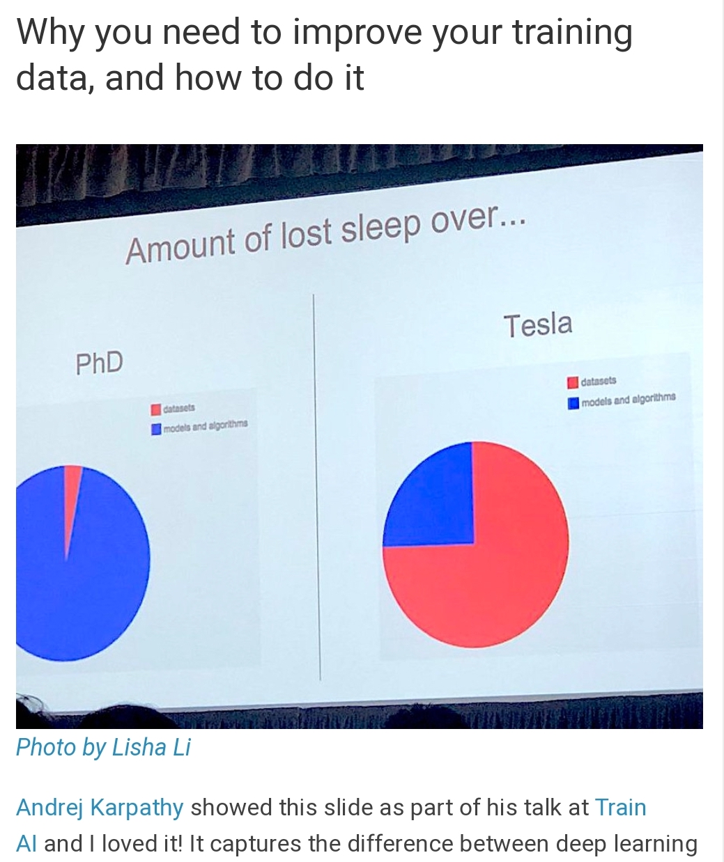
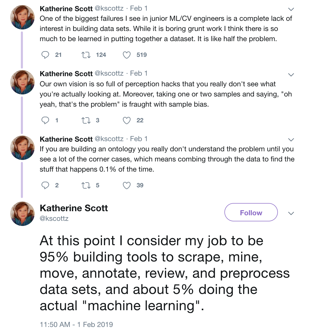
- "scrape, mine, move, annotate, review, and preprocess" - Kathy Scott
- tools to use
- simulation
Augmentation
- How can you artifically increase the size of your dataset?
- What are the limits of these increases
Baselines
- What is a baseline?
- Nearest Neighbor
- Linear Models
Reproducibility
- Version Control
- Data Versioning
References
Revisiting Unreasonable Effectiveness of Data in Deep Learning Era: https://arxiv.org/abs/1707.02968
Building Datasets
- Python Machine Learning 2nd Edition by Sebastian Raschka, Packt Publishing Ltd. 2017
- Chapter 2: Building Good Datasets: https://github.com/rasbt/python-machine-learning-book-2nd-edition/blob/master/code/ch04/ch04.ipynb
- A Standardised Approach for Preparing Imaging Data for Machine Learning Tasks in Radiology https://link.springer.com/chapter/10.1007/978-3-319-94878-2_6
Creating Datasets / Crowdsourcing
Mindcontrol: A web application for brain segmentation quality control: https://www.sciencedirect.com/science/article/pii/S1053811917302707
Combining citizen science and deep learning to amplify expertise in neuroimaging: https://www.biorxiv.org/content/10.1101/363382v1.abstract
Versioning Datasets
Augmentation
Reproducibility
Trouble at the lab Scientists like to think of science as self-correcting. To an alarming degree, it is not
Why is reproducible research important? The Real Reason Reproducible Research is Important
Reproducible Research Class @ Johns Hopkins University
Who am I?
Kevin Mader (mader@biomed.ee.ethz.ch)
Deep Learning Software Engineer at Magic Leap
Cofounder of 4Quant for Big Image Analytics (ETH Spin-off, 2013-2018)
Lecturer at ETH Zurich (2013-2019)
Formerly Postdoc in the X-Ray Microscopy Group at ETH Zurich (2013-2015)
PhD Student at Swiss Light Source at Paul Scherrer Institute (2008-2012)

Motivation
Most of you taking this class are rightfully excited to learn about new tools and algorithms to analyzing your data. This lecture is a bit of an anomaly and perhaps disappointment because it doesn't cover any algorithms, or tools.
- So you might ask, why are we spending so much time on datasets?
- You already collected data (sometimes lots of it) that is why you took this class?!

Data is important
It probably isn't the new oil, but it forms an essential component for building modern tools today.
Testing good algorithms requires good data
If you don't know what to expect how do you know your algorithm worked?
If you have dozens of edge cases how can you make sure it works on each one?
If a new algorithm is developed every few hours, how can you be confident they actually work better (facebook's site has a new version multiple times per day and their app every other day)
For machine learning, even building requires good data
If you count cells maybe you can write your own algorithm,
but if you are trying to detect subtle changes in cell structure that indicate cancer you probably can't write a list of simple mathematical rules yourself.
Data is reusable
Well organized and structure data is very easy to reuse. Another project can easily combine your data with their data in order to get even better results.
- Algorithms are messy, complicated, poorly written, ... (especially so if written by students trying to graduate on time)
Famous Datasets
The primary success of datasets has been shown through the most famous datasets collected. Here I show 2 of the most famous general datasets and one of the most famous medical datasets. The famous datasets are important for
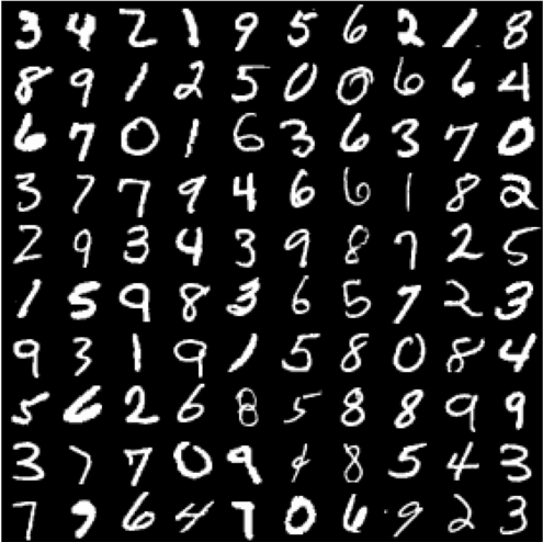
- MNIST Digits
- Modified NIST (National Institute of Standards and Technology) created a list of handwritten digits
- ImageNet
- ImageNet is an image database organized according to the WordNet hierarchy (currently only the nouns), in which each node of the hierarchy is depicted by hundreds and thousands of images.
- 1000 different categories and >1M images.
- Not just dog/cat, but wolf vs german shepard,
- BRATS
- Segmenting Tumors in Multimodal MRI Brain Images.
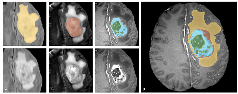
What story did these datasets tell?
Each of these datasets is very different from images with fewer than 1000 pixels to images with more than 100MPx, but what they have in common is how their analysis has changed.
Hand-crafted features
All of these datasets used to be analyzed by domain experts with hand-crafted features.
- A handwriting expert using graph topology to assign images to digits
- A computer vision expert using gradients common in faces to identify people in ImageNet
- A biomedical engineer using knowledge of different modalities to fuse them together and cluster healthy and tumorous tissue
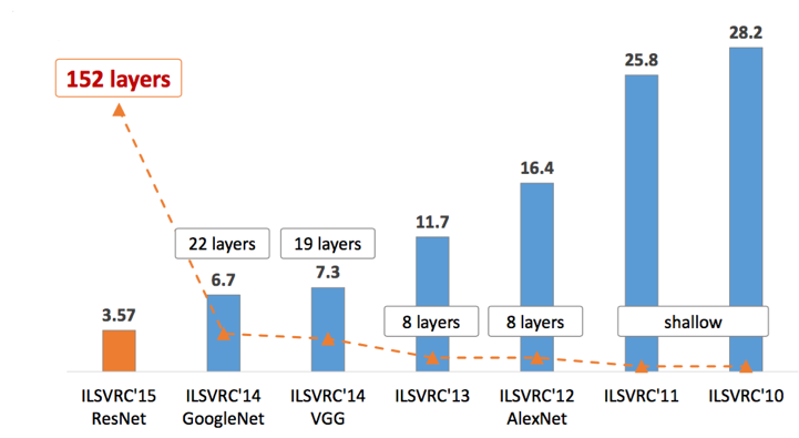
Machine Learning / Deep Learning
Starting in the early 2010s, the approaches of deep learning began to improve and become more computationally efficient. With these techniques groups with absolutely no domain knowledge could begin building algorithms and winning contests based on these datasets
So Deep Learning always wins?
No, that isn't the point of this lecture. Even if you aren't using deep learning the point of these stories is having well-labeled, structured, and organized datasets makes your problem a lot more accessible for other groups and enables a variety of different approaches to be tried. Ultimately it enables better solutions to be made and you to be confident that the solutions are in fact better
Other Datasets
- Grand-Challenge.org a large number of challenges in the biomedical area
- Kaggle Datasets
- Google Dataset Search
- The Cancer Imaging Archive (multi-modal medical data)
What makes a good dataset?
- Lots of images
- Small datasets can be useful but here the bigger the better
- Particularly if you have complicated problems and/or very subtle differences (ie a lung tumor looks mostly like normal lung tissue but it is in a place it shouldn't be)
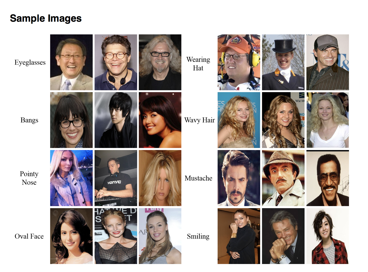
- Lots of diversity
- Is it what data 'in the wild' really looks like?
- Lots of different scanners/reconstruction algorithms, noise, illumination types, rotation, colors, ...
- Many examples from different categories (if you only have one male with breast cancer it will be hard to generalize exactly what that looks like)
- Meaningful labels
- Clear task or question
- Unambiguous (would multiple different labelers come to the same conclusion)
- Able to be derived from the image alone (a label that someone cannot afford insurance is interesting but it would be nearly impossible to determine that from an X-ray of their lungs)
- Quantitative!
- Non-obvious (a label saying an image is bright is not a helpful label because you could look at the histogram and say that)
Types of Datasets
- Classification
- Regression
- Segmentation
- Detection
- Other
Classification
- Taking an image and putting it into a category
- Each image should have exactly one category
- The categories should be non-ordered
- Example:
- Cat vs Dog
- Cancer vs Healthy
import numpy as np
import matplotlib.pyplot as plt
from keras.datasets import mnist
from skimage.util import montage as montage2d
%matplotlib inline
(img, label), _ = mnist.load_data()
fig, m_axs = plt.subplots(5, 5, figsize=(9, 9))
for c_ax, c_img, c_label in zip(m_axs.flatten(), img, label):
    c_ax.imshow(c_img, cmap='gray')
    c_ax.set_title(c_label)
    c_ax.axis('off')
/Users/kevinmader/miniconda3/envs/qbi2019/lib/python3.6/site-packages/h5py/__init__.py:36: FutureWarning: Conversion of the second argument of issubdtype from `float` to `np.floating` is deprecated. In future, it will be treated as `np.float64 == np.dtype(float).type`.
  from ._conv import register_converters as _register_converters
Using TensorFlow backend.

Regression
- Taking an image and predicting one (or more) decimal values
- Examples:
- Value of a house from the picture taken by owner
- Risk of hurricane from satellite image

Segmentation
- Taking an image and predicting one (or more) values for each pixel
- Every pixel needs a label (and a pixel cannot have multiple labels)
- Typically limited to a few (<20) different types of objects
- Examples:
- Where a tumor is from an image of the lungs
- Where streets are from satellite images of a neighborhood
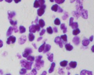
Nuclei in Microscope Images

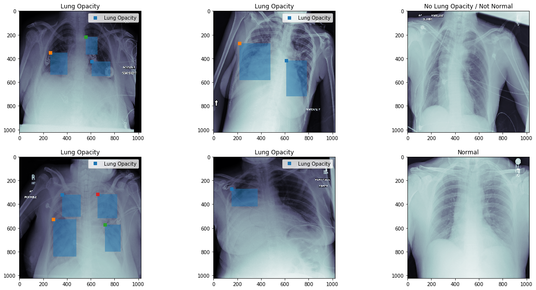
Detection
- Taking an image and predicting where and which type of objects appear
- Generally bounding box rather then specific pixels
- Multiple objects can overlap
Opaque Regions in X-Rays
Other
- Unlimited possibilities here
- Horses to Zebras
Image Enhancement
- Denoising Learning to See in the Dark
- Super-resolution
Building your own
- Very time consuming
- Not a lot of great tools
- Very problem specific
- Free tools
- Classification / Segmentation: https://github.com/Labelbox/Labelbox
- Classification/ Object Detection: http://labelme.csail.mit.edu/Release3.0/
- Classification: https://github.com/janfreyberg/superintendent: https://www.youtube.com/watch?v=fMg0mPYiEx0
- Classification/ Detection: https://github.com/chestrays/jupyanno: https://www.youtube.com/watch?v=XDIJU5Beg_w
- Classification (Tinder for Brain MRI): https://braindr.us/#/
- Commercial Approaches
- https://www.figure-eight.com/
- MightyAI / Spare5: https://mighty.ai/ https://app.spare5.com/fives/sign_in
Dataset Problems
Some of the issues which can come up with datasets are
- imbalance
- too few examples
- too homogenous
- and other possible problems
These lead to problems with the algorithms built on top of them.
Bias

Google Photos, y'all *** up. My friend's not a gorilla. pic.twitter.com/SMkMCsNVX4
— I post from https://v2.jacky.wtf. 🆓 != safe. (@jackyalcine) June 29, 2015
- Solution was to remove Gorilla from the category (https://www.theverge.com/2018/1/12/16882408/google-racist-gorillas-photo-recognition-algorithm-ai)
import numpy as np
import matplotlib.pyplot as plt
from keras.datasets import mnist
from skimage.util import montage as montage2d
%matplotlib inline
(img, label), _ = mnist.load_data()

fig, (ax1, ax2) = plt.subplots(1, 2, figsize=(16,  8))
d_subset = np.where(np.in1d(label, [1, 2, 3]))[0]
ax1.imshow(montage2d(img[d_subset[:64]]), cmap='gray')
ax1.set_title('Images')
ax1.axis('off')
ax2.hist(label[d_subset[:64]], np.arange(11))
ax2.set_title('Digit Distribution')
Text(0.5, 1.0, 'Digit Distribution')

Augmentation
Most groups have too little well-labeled data and labeling new examples can be very expensive. Additionally there might not be very many cases of specific classes. In medicine this is particularly problematic, because some diseases might only happen a few times in a given hospital and you still want to be able to recognize the disease and not that particular person.
Transformation
- Shift
- Zoom
- Rotation
- Intensity
- Normalization
- Scaling
- Color
- Shear
Limitations
- What transformations are normal in the images?
- CT images usually do not get flipped (the head is always on the top)
- The values in CT images have a physical meaning (Hounsfield unit), scaling them changes the image
- How much distortion is too much?
- Can you still recognize the features?
ImageDataGenerator(
    ['featurewise_center=False', 'samplewise_center=False', 'featurewise_std_normalization=False', 'samplewise_std_normalization=False', 'zca_whitening=False', 'zca_epsilon=1e-06', 'rotation_range=0.0', 'width_shift_range=0.0', 'height_shift_range=0.0', 'shear_range=0.0', 'zoom_range=0.0', 'channel_shift_range=0.0', "fill_mode='nearest'", 'cval=0.0', 'horizontal_flip=False', 'vertical_flip=False', 'rescale=None', 'preprocessing_function=None', 'data_format=None'],
)
Docstring:
Generate minibatches of image data with real-time data augmentation.

# Arguments
    featurewise_center: set input mean to 0 over the dataset.
    samplewise_center: set each sample mean to 0.
    featurewise_std_normalization: divide inputs by std of the dataset.
    samplewise_std_normalization: divide each input by its std.
    zca_whitening: apply ZCA whitening.
    zca_epsilon: epsilon for ZCA whitening. Default is 1e-6.
    rotation_range: degrees (0 to 180).
    width_shift_range: fraction of total width, if < 1, or pixels if >= 1.
    height_shift_range: fraction of total height, if < 1, or pixels if >= 1.
    shear_range: shear intensity (shear angle in degrees).
    zoom_range: amount of zoom. if scalar z, zoom will be randomly picked
        in the range [1-z, 1+z]. A sequence of two can be passed instead
        to select this range.
    channel_shift_range: shift range for each channel.
    fill_mode: points outside the boundaries are filled according to the
        given mode ('constant', 'nearest', 'reflect' or 'wrap'). Default
        is 'nearest'.
        Points outside the boundaries of the input are filled according to the given mode:
            'constant': kkkkkkkk|abcd|kkkkkkkk (cval=k)
            'nearest':  aaaaaaaa|abcd|dddddddd
            'reflect':  abcddcba|abcd|dcbaabcd
            'wrap':  abcdabcd|abcd|abcdabcd
    cval: value used for points outside the boundaries when fill_mode is
        'constant'. Default is 0.
    horizontal_flip: whether to randomly flip images horizontally.
    vertical_flip: whether to randomly flip images vertically.
    rescale: rescaling factor. If None or 0, no rescaling is applied,
        otherwise we multiply the data by the value provided. This is
        applied after the `preprocessing_function` (if any provided)
        but before any other transformation.
    preprocessing_function: function that will be implied on each input.
        The function will run before any other modification on it.
        The function should take one argument:
        one image (Numpy tensor with rank 3),
from keras.preprocessing.image import ImageDataGenerator
img_aug = ImageDataGenerator(
    featurewise_center=False,
    samplewise_center=False,
    zca_whitening=False,
    zca_epsilon=1e-06,
    rotation_range=30.0,
    width_shift_range=0.25,
    height_shift_range=0.25,
    shear_range=0.25,
    zoom_range=0.5,
    fill_mode='nearest',
    horizontal_flip=False,
    vertical_flip=False
)
MNIST
Even something as simple as labeling digits can be very time consuming (maybe 1-2 per second).
import numpy as np
import matplotlib.pyplot as plt
from keras.datasets import mnist
%matplotlib inline
(img, label), _ = mnist.load_data()
img = np.expand_dims(img, -1)
fig, m_axs = plt.subplots(4, 10, figsize=(16, 10))
# setup augmentation
img_aug.fit(img)
real_aug = img_aug.flow(img[:10], label[:10], shuffle=False)
for c_axs, do_augmentation in zip(m_axs, [False, True, True, True]):
    if do_augmentation:
        img_batch, label_batch = next(real_aug)
    else:
        img_batch, label_batch = img, label
    for c_ax, c_img, c_label in zip(c_axs, img_batch, label_batch):
        c_ax.imshow(c_img[:, :, 0], cmap='gray', vmin=0, vmax=255)
        c_ax.set_title('{}\n{}'.format(
            c_label, 'aug' if do_augmentation else ''))
        c_ax.axis('off')

CIFAR10
We can use a more exciting dataset to try some of the other features in augmentation
from keras.datasets import cifar10
(img, label), _ = cifar10.load_data()
img_aug = ImageDataGenerator(
    featurewise_center=True,
    samplewise_center=False,
    zca_whitening=False,
    zca_epsilon=1e-06,
    rotation_range=30.0,
    width_shift_range=0.25,
    height_shift_range=0.25,
    channel_shift_range=0.25,
    shear_range=0.25,
    zoom_range=1,
    fill_mode='reflect',
    horizontal_flip=True,
    vertical_flip=True
)
import numpy as np
import matplotlib.pyplot as plt
from keras.datasets import mnist
%matplotlib inline
fig, m_axs = plt.subplots(4, 10, figsize=(16, 12))
# setup augmentation
img_aug.fit(img)
real_aug = img_aug.flow(img[:10], label[:10], shuffle=False)
for c_axs, do_augmentation in zip(m_axs, [False, True, True, True]):
    if do_augmentation:
        img_batch, label_batch = next(real_aug)
        img_batch -= img_batch.min()
        img_batch = np.clip(img_batch/img_batch.max() *
                            255, 0, 255).astype('uint8')
    else:
        img_batch, label_batch = img, label
    for c_ax, c_img, c_label in zip(c_axs, img_batch, label_batch):
        c_ax.imshow(c_img)
        c_ax.set_title('{}\n{}'.format(
            c_label[0], 'aug' if do_augmentation else ''))
        c_ax.axis('off')

Basic Models Overview
There are a number of methods we can use for classification, regression and both. For the simplification of the material we will not make a massive distinction between classification and regression but there are many situations where this is not appropriate. Here we cover a few basic methods, since these are important to understand as a starting point for solving difficult problems. The list is not complete and importantly Support Vector Machines are completely missing which can be a very useful tool in supervised analysis. A core idea to supervised models is they have a training phase and a predicting phase.
Training
The training phase is when the parameters of the model are learned and involve putting inputs into the model and updating the parameters so they better match the outputs. This is a sort-of curve fitting (with linear regression it is exactly curve fitting).
Predicting
The predicting phase is once the parameters have been set applying the model to new datasets. At this point the parameters are no longer adjusted or updated and the model is frozen. Generally it is not possible to tweak a model any more using new data but some approaches (most notably neural networks) are able to handle this.
Baselines
- A baseline is a simple, easily implemented and understood model that illustrates the problem and the 'worst-case scenerio' for a model that learns nothing (some models will do worse, but these are especially useless).
- Why is this important?
- I have a a model that is >99% accurate for predicting breast cancer
- Breast Cancer incidence is $\approx$ 89 of 100,000 women (0.09%) so always saying no has an accuracy of 99.91%
from sklearn.dummy import DummyClassifier
dc = DummyClassifier(strategy='most_frequent')
dc.fit([0, 1, 2, 3],
       ['Healthy', 'Healthy', 'Healthy', 'Cancer'])
DummyClassifier(constant=None, random_state=None, strategy='most_frequent')
dc.predict([0]), dc.predict([1]), dc.predict([3]), dc.predict([100])
(array(['Healthy'], dtype='<U7'),
 array(['Healthy'], dtype='<U7'),
 array(['Healthy'], dtype='<U7'),
 array(['Healthy'], dtype='<U7'))
Simple Toy Problems
Rather than jumping right into the sort of datasets we looked at before, we focus on a simple 2D problem which we can easily visualize and understand. Here we have clusters of colored points.
import pandas as pd
import numpy as np
import matplotlib.pyplot as plt
from sklearn.datasets import make_blobs
%matplotlib inline

blob_data, blob_labels = make_blobs(n_samples=200,
                                    cluster_std=2.0,
                                    random_state=2018)
test_pts = pd.DataFrame(blob_data, columns=['x', 'y'])
test_pts['group_id'] = blob_labels
plt.scatter(test_pts.x, test_pts.y,
            c=test_pts.group_id,
            cmap='viridis')
test_pts.sample(5)
| x | y | group_id | |
|---|---|---|---|
| 72 | -1.100380 | 0.794467 | 2 |
| 48 | 8.388243 | -11.122531 | 0 |
| 69 | 8.947938 | -8.774467 | 0 |
| 105 | 4.943428 | -6.820184 | 0 |
| 27 | -0.286168 | 3.292601 | 2 |

Nearest Neighbor (or K Nearest Neighbors)
The technique is as basic as it sounds, it basically finds the nearest point to what you have put in.
from sklearn.neighbors import KNeighborsClassifier
import numpy as np
k_class = KNeighborsClassifier(1)
k_class.fit(X=np.reshape([0, 1, 2, 3], (-1, 1)),
            y=['I', 'am', 'a', 'dog'])
KNeighborsClassifier(algorithm='auto', leaf_size=30, metric='minkowski',
           metric_params=None, n_jobs=None, n_neighbors=1, p=2,
           weights='uniform')
print(
    k_class.predict(
        np.reshape([0, 1, 2, 3], (-1, 1))
    )
)
['I' 'am' 'a' 'dog']
print(
    k_class.predict(
        np.reshape([1.5], (1, 1))
    )
)
print(
    k_class.predict(
        np.reshape([100], (1, 1))
    )
)
['am']
['dog']
k_class = KNeighborsClassifier(1)
k_class.fit(test_pts[['x', 'y']], test_pts['group_id'])
KNeighborsClassifier(algorithm='auto', leaf_size=30, metric='minkowski',
           metric_params=None, n_jobs=None, n_neighbors=1, p=2,
           weights='uniform')
xx, yy = np.meshgrid(np.linspace(test_pts.x.min(), test_pts.x.max(), 30),
                     np.linspace(test_pts.y.min(), test_pts.y.max(), 30),
                     indexing='ij'
                     )
grid_pts = pd.DataFrame(dict(x=xx.ravel(), y=yy.ravel()))
grid_pts['predicted_id'] = k_class.predict(grid_pts[['x', 'y']])

fig, (ax1, ax2) = plt.subplots(2, 1, figsize=(6, 12))
ax1.scatter(test_pts.x, test_pts.y, c=test_pts.group_id, cmap='viridis')
ax1.set_title('Training Data')
ax2.scatter(grid_pts.x, grid_pts.y, c=grid_pts.predicted_id, cmap='viridis')
ax2.set_title('Testing Points')
Text(0.5, 1.0, 'Testing Points')

Stabilizing Results
We can see here that the result is thrown off by single points, we can improve by using more than the nearest neighbor and include the average of the nearest 2 neighbors.
k_class = KNeighborsClassifier(3)
k_class.fit(test_pts[['x', 'y']], test_pts['group_id'])
xx, yy = np.meshgrid(np.linspace(test_pts.x.min(), test_pts.x.max(), 30),
                     np.linspace(test_pts.y.min(), test_pts.y.max(), 30),
                     indexing='ij'
                     )
grid_pts = pd.DataFrame(dict(x=xx.ravel(),
                             y=yy.ravel()))
grid_pts['predicted_id'] = k_class.predict(grid_pts[['x', 'y']])

fig, (ax1, ax2) = plt.subplots(2, 1, figsize=(6, 12))
ax1.scatter(test_pts.x, test_pts.y, c=test_pts.group_id, cmap='viridis')
ax1.set_title('Training Data')
ax2.scatter(grid_pts.x, grid_pts.y, c=grid_pts.predicted_id, cmap='viridis')
ax2.set_title('Testing Points')
Text(0.5, 1.0, 'Testing Points')

Logistic Regression
So logistic regression is linear regression adapted for classification. Instead of predicting a linear output we predict a dichotomous variable.
from sklearn.linear_model import LogisticRegression
log_reg = LogisticRegression(solver='lbfgs', multi_class='auto')
log_reg.fit(test_pts[['x', 'y']], test_pts['group_id'])
xx, yy = np.meshgrid(np.linspace(test_pts.x.min(), test_pts.x.max(), 30),
                     np.linspace(test_pts.y.min(), test_pts.y.max(), 30),
                     indexing='ij'
                     )
grid_pts = pd.DataFrame(dict(x=xx.ravel(),
                             y=yy.ravel()))
grid_pts['predicted_id'] = log_reg.predict(grid_pts[['x', 'y']])

fig, ((ax1, ax2, ax3), b_axs) = plt.subplots(2, 3, figsize=(12, 8))
ax1.scatter(test_pts.x, test_pts.y, c=test_pts.group_id, cmap='viridis')
ax1.set_title('Training Data')
ax2.scatter(grid_pts.x, grid_pts.y, c=grid_pts.predicted_id, cmap='viridis')
ax2.set_title('Testing Points')
ax3.axis('off')
for i, c_ax in enumerate(b_axs):
    c_prob = log_reg.predict_proba(grid_pts[['x', 'y']])[:, i]
    c_plot = c_ax.scatter(grid_pts.x, grid_pts.y, c=c_prob,
                          cmap='magma', vmin=0, vmax=1)
    c_ax.set_title('Class #{} probability'.format(i))
plt.colorbar(c_plot);

Trees and Forests
Decision Tree
Taking a problem and dividing it into a number of yes/no questions based on individual variables that are followed in a specified order. A decision tree for likelihood for getting Manchester United Football tickets might look like follow
- Are you a member of the ManU fan club (Yes -> go to 2, No -> go to 3)
- Probability of getting tickets 90%
- Are you willing to spend more than 1000CHF (Yes -> go to 4, No -> go to 5)
- Probability of getting tickets 80%
- Are you a famous celebrity (Yes -> go to 6, No -> go to 7)
- Probability of getting tickets 90%
- Probability of getting tickets 10%
Forests
Basically the idea of taking a number of trees and bringing them together. So rather than taking a single tree to do the classification, you divide the samples and the features to make different trees and then combine the results. One of the more successful approaches is called Random Forests or as a video
from sklearn.tree import export_graphviz
import graphviz
from sklearn.tree import DecisionTreeClassifier
import numpy as np

def show_tree(in_tree):
    return graphviz.Source(export_graphviz(in_tree, out_file=None))

d_tree = DecisionTreeClassifier()
d_tree.fit(X=np.reshape([0, 1, 2, 3], (-1, 1)),
           y=[0, 1, 0, 1])
show_tree(d_tree)
d_tree = DecisionTreeClassifier()
d_tree.fit(test_pts[['x', 'y']],
           test_pts['group_id'])
show_tree(d_tree)
xx, yy = np.meshgrid(np.linspace(test_pts.x.min(), test_pts.x.max(), 40),
                     np.linspace(test_pts.y.min(), test_pts.y.max(), 40),
                     indexing='ij'
                     )
grid_pts = pd.DataFrame(dict(x=xx.ravel(), y=yy.ravel()))
grid_pts['predicted_id'] = d_tree.predict(grid_pts[['x', 'y']])

fig, (ax1, ax2) = plt.subplots(1, 2, figsize=(12, 4))
ax1.scatter(test_pts.x, test_pts.y, c=test_pts.group_id, cmap='viridis')
ax1.set_title('Training Data')
ax2.scatter(grid_pts.x, grid_pts.y, c=grid_pts.predicted_id, cmap='viridis')
ax2.set_title('Testing Points')
Text(0.5, 1.0, 'Testing Points')

from sklearn.ensemble import RandomForestClassifier
rf_class = RandomForestClassifier(n_estimators=5, random_state=2018)
rf_class.fit(test_pts[['x', 'y']],
             test_pts['group_id'])
print('Build ', len(rf_class.estimators_), 'decision trees')
Build 5 decision trees
show_tree(rf_class.estimators_[0])
xx, yy = np.meshgrid(np.linspace(test_pts.x.min(), test_pts.x.max(), 50),
                     np.linspace(test_pts.y.min(), test_pts.y.max(), 50),
                     indexing='ij'
                     )
grid_pts = pd.DataFrame(dict(x=xx.ravel(), y=yy.ravel()))

fig, (ax1, ax2, ax3, ax4) = plt.subplots(1, 4, figsize=(14, 3), dpi=150)
ax1.scatter(test_pts.x, test_pts.y, c=test_pts.group_id, cmap='viridis')
ax1.set_title('Training Data')
ax2.scatter(grid_pts.x, grid_pts.y, c=rf_class.predict(
    grid_pts[['x', 'y']]), cmap='viridis')
ax2.set_title('Random Forest Classifier')

ax3.scatter(grid_pts.x, grid_pts.y, c=rf_class.estimators_[
            0].predict(grid_pts[['x', 'y']]), cmap='viridis')
ax3.set_title('First Decision Tree')

ax4.scatter(grid_pts.x, grid_pts.y, c=rf_class.estimators_[
            1].predict(grid_pts[['x', 'y']]), cmap='viridis')
ax4.set_title('Second Decision Tree')
Text(0.5, 1.0, 'Second Decision Tree')

fig, b_axs = plt.subplots(1, 3, figsize=(12, 4))
for i, c_ax in enumerate(b_axs):
    c_prob = rf_class.predict_proba(grid_pts[['x', 'y']])[:, i]
    c_plot = c_ax.scatter(grid_pts.x, grid_pts.y, c=c_prob,
                          cmap='magma', vmin=0, vmax=1)
    c_ax.set_title('Class #{} probability'.format(i))
plt.colorbar(c_plot);

Applying to Digit Classification
We have now spent enough time building these models on toy problems we can now apply them again to Digit Classification to understand what kind of information a baseline model can give us.
import numpy as np
import matplotlib.pyplot as plt
from keras.datasets import mnist
from skimage.util import montage as montage2d
%matplotlib inline
(img, label), _ = mnist.load_data()
fig, m_axs = plt.subplots(5, 5, figsize=(12, 12))
m_axs[0, 0].hist(label[:24], np.arange(11))
m_axs[0, 0].set_title('Digit Distribution')
for i, c_ax in enumerate(m_axs.flatten()[1:]):
    c_ax.imshow(img[i], cmap='gray')
    c_ax.set_title(label[i])
    c_ax.axis('off')

dc = DummyClassifier(strategy='most_frequent')
dc.fit(img[:24], label[:24])
DummyClassifier(constant=None, random_state=None, strategy='most_frequent')
dc.predict(img[0:10])
array([1, 1, 1, 1, 1, 1, 1, 1, 1, 1], dtype=uint8)
fig, m_axs = plt.subplots(4, 6, figsize=(12, 12))
for i, c_ax in enumerate(m_axs.flatten()):
    c_ax.imshow(img[i], cmap='gray')
    c_ax.set_title('{}\nPredicted: {}'.format(label[i], dc.predict(img[i])[0]))
    c_ax.axis('off')

Nearest Neighbor
This isn't a machine learning class and so we won't dive deeply into other methods, but nearest neighbor is often a very good baseline (that is also very easy to understand). You basically take the element from the original set that is closest to the image you show.
- You can make the method more robust by using more than one nearest neighbor (hence K nearest neighbors), but that we will cover in the supervised methods lecture
import numpy as np
import matplotlib.pyplot as plt
from keras.datasets import mnist
from skimage.util import montage as montage2d
%matplotlib inline
(img, label), _ = mnist.load_data()
fig, m_axs = plt.subplots(5, 5, figsize=(12, 12))
m_axs[0, 0].hist(label[:24], np.arange(11))
m_axs[0, 0].set_title('Digit Distribution')
for i, c_ax in enumerate(m_axs.flatten()[1:]):
    c_ax.imshow(img[i], cmap='gray')
    c_ax.set_title(label[i])
    c_ax.axis('off')
from sklearn.neighbors import KNeighborsClassifier
neigh_class = KNeighborsClassifier(n_neighbors=1)
neigh_class.fit(img[:24].reshape((24, -1)), label[:24])
KNeighborsClassifier(algorithm='auto', leaf_size=30, metric='minkowski',
           metric_params=None, n_jobs=None, n_neighbors=1, p=2,
           weights='uniform')
# predict on a few images
neigh_class.predict(img[0:10].reshape((10, -1)))
array([5, 0, 4, 1, 9, 2, 1, 3, 1, 4], dtype=uint8)
fig, m_axs = plt.subplots(4, 6, figsize=(12, 12))
for i, c_ax in enumerate(m_axs.flatten()):
    c_ax.imshow(img[i], cmap='gray')
    c_ax.set_title('{}\nPredicted: {}'.format(label[i],
                                              neigh_class.predict(img[i].reshape((1, -1)))[0]))
    c_ax.axis('off')

100% for a baseline
Wow the model works really really well, it got every example perfectly. What we did here (a common mistake) was evaluate on the same data we 'trained' on which means the model just correctly recalled each example, if we try it on new images we can see the performance drop but still a reasonable result
fig, m_axs = plt.subplots(4, 6, figsize=(12, 12))
for i, c_ax in enumerate(m_axs.flatten(), 25):
    c_ax.imshow(img[i], cmap='gray')
    c_ax.set_title('{}\nPredicted: {}'.format(label[i],
                                              neigh_class.predict(img[i].reshape((1, -1)))[0]))
    c_ax.axis('off')

import seaborn as sns
import pandas as pd


def print_confusion_matrix(confusion_matrix, class_names, figsize=(10, 7), fontsize=14):
    """Prints a confusion matrix, as returned by sklearn.metrics.confusion_matrix, as a heatmap.

    Stolen from: https://gist.github.com/shaypal5/94c53d765083101efc0240d776a23823

    Arguments
    ---------
    confusion_matrix: numpy.ndarray
        The numpy.ndarray object returned from a call to sklearn.metrics.confusion_matrix.
        Similarly constructed ndarrays can also be used.
    class_names: list
        An ordered list of class names, in the order they index the given confusion matrix.
    figsize: tuple
        A 2-long tuple, the first value determining the horizontal size of the ouputted figure,
        the second determining the vertical size. Defaults to (10,7).
    fontsize: int
        Font size for axes labels. Defaults to 14.

    Returns
    -------
    matplotlib.figure.Figure
        The resulting confusion matrix figure
    """
    df_cm = pd.DataFrame(
        confusion_matrix, index=class_names, columns=class_names,
    )
    fig, ax1 = plt.subplots(1, 1, figsize=figsize)
    try:
        heatmap = sns.heatmap(df_cm, annot=True, fmt="d")
    except ValueError:
        raise ValueError("Confusion matrix values must be integers.")
    heatmap.yaxis.set_ticklabels(
        heatmap.yaxis.get_ticklabels(), rotation=0, ha='right', fontsize=fontsize)
    heatmap.xaxis.set_ticklabels(
        heatmap.xaxis.get_ticklabels(), rotation=45, ha='right', fontsize=fontsize)
    plt.ylabel('True label')
    plt.xlabel('Predicted label')
    return ax1
from sklearn.metrics import accuracy_score, confusion_matrix
train_img_count = 1000
neigh_class.fit(img[:train_img_count].reshape((train_img_count, -1)),
                label[:train_img_count])
pred_values = neigh_class.predict(img[train_img_count:].reshape((-1, 28*28)))
ax1 = print_confusion_matrix(
    confusion_matrix(
        label[train_img_count:],
        pred_values),
    class_names=range(10))
ax1.set_title('Accuracy: {:2.2%}'.format(
    accuracy_score(label[train_img_count:],
                   pred_values)))
Text(0.5, 1.0, 'Accuracy: 86.93%')

Random Forest
rf_class = RandomForestClassifier(n_estimators=100,
                                  random_state=2018)
rf_class.fit(img[:train_img_count].reshape((train_img_count, -1)),
             label[:train_img_count])
RandomForestClassifier(bootstrap=True, class_weight=None, criterion='gini',
            max_depth=None, max_features='auto', max_leaf_nodes=None,
            min_impurity_decrease=0.0, min_impurity_split=None,
            min_samples_leaf=1, min_samples_split=2,
            min_weight_fraction_leaf=0.0, n_estimators=100, n_jobs=None,
            oob_score=False, random_state=2018, verbose=0,
            warm_start=False)
pred_values = rf_class.predict(img[train_img_count:].reshape((-1, 28*28)))
ax1 = print_confusion_matrix(confusion_matrix(
    label[train_img_count:], pred_values),
                             class_names=range(10))
ax1.set_title('Accuracy: {:2.2%}'.format(
    accuracy_score(label[train_img_count:], pred_values)));

Science and Imaging
Images are great for qualitative analyses since our brains can quickly interpret them without large programming investements.
Proper processing and quantitative analysis is however much more difficult with images.
- If you measure a temperature, quantitative analysis is easy, $50K$.
- If you measure an image it is much more difficult and much more prone to mistakes, subtle setup variations, and confusing analyses
Furthermore in image processing there is a plethora of tools available
- Thousands of algorithms available
- Thousands of tools
- Many images require multi-step processing
- Experimenting is time-consuming
Reproducibility
Science demands repeatability! and really wants reproducability
- Experimental conditions can change rapidly and are difficult to make consistent
- Animal and human studies are prohibitively time consuming and expensive to reproduce
- Terabyte datasets cannot be easily passed around many different groups
- Privacy concerns can also limit sharing and access to data
- Science is already difficult enough
- Image processing makes it even more complicated
- Many image processing tasks are multistep, have many parameters, use a variety of tools, and consume a very long time
Version Control
Like track-changes in word processing software, you can track changes across code using tools called version control. Websites like GitHub, GitLab, and Bitbucket make this very easy to do and every modern software engineer uses these tools daily for all kinds of large and small projects.
Data Version Control
Just like code you can track changes in your data and labels and these are often even more important to track well. Tools like DVC make this much easier to do for projects and scale well to millions of images and labels.