Undamped Response to Harmonic Direct-Force Inputs
MCHE 485: Mechanical Vibrations
Dr. Joshua Vaughan
joshua.vaughan@louisiana.edu
http://www.ucs.louisiana.edu/~jev9637/
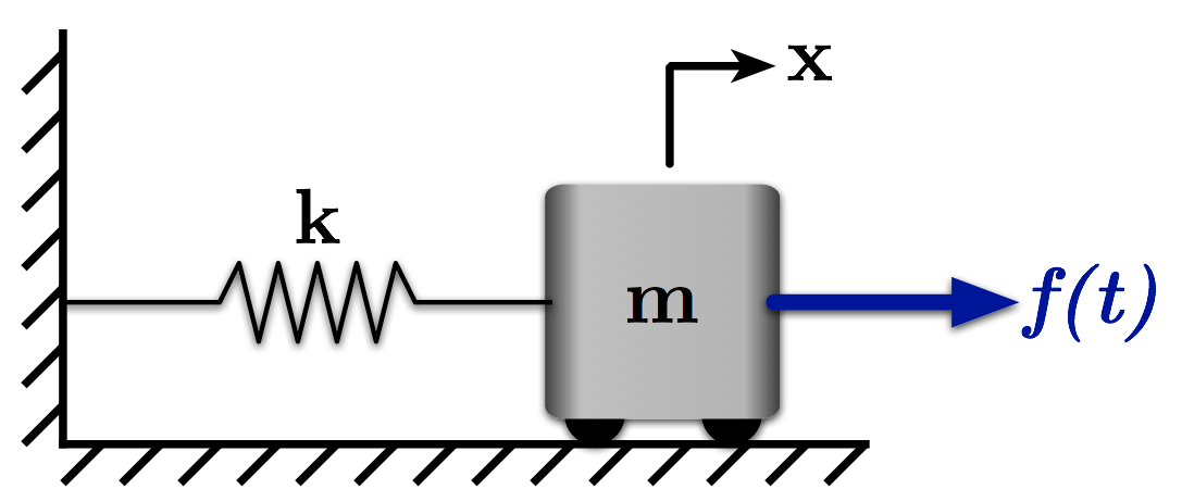
Figure 1: A Mass-Spring System
This notebook examines the frequency response of a simple mass-spring system like the one shown in Figure 1 to a harmonic, direct-force input.
The equation of motion for the system is:
$ \quad m \ddot{x} + kx = f $
We could also write this equation in terms of the damping ratio, $\zeta$, and natural frequency, $\omega_n$.
$ \quad \ddot{x} + \omega_n^2x = \frac{f}{m}$
For information on how to obtain this equation, you can see the lectures at the class website.
import numpy as np # Grab all of the NumPy functions with nickname np
# We want our plots to be displayed inline, not in a separate window
%matplotlib inline
# Import the plotting functions
import matplotlib.pyplot as plt
# Define the System Parameters
m = 1.0                 # kg
k = (2.0 * np.pi)**2.      # N/m (Selected to give an undamped natrual frequency of 1Hz)
wn = np.sqrt(k / m)       # Natural Frequency (rad/s)
Let's use the closed-form, steady-state solution we developed in lecture:
Assume:
$ \quad f(t) = \bar{f} \sin{\omega t} $
Then, the solution $x(t)$ should have the form:
$ \quad x(t) = \bar{x} \sin{\omega t} $
We can then find the amplitude of the frequency response, $ \bar{x} $, as a function of of the frequency of the input, $ \omega $, and the amplitude of the force, $ \bar{f} $.
$ \quad \bar{x} = \frac{\bar{f}}{m} \left(\frac{1}{\omega_n^2 - \omega^2}\right) $
So,
$ \quad x(t) = \frac{\bar{f}}{m} \left(\frac{1}{\omega_n^2 - \omega^2}\right) \sin{\omega t} $
or
$ \quad x(t) = \frac{1}{m} \left(\frac{1}{\omega_n^2 - \omega^2} \right) f(t) $
So, $ \left(\frac{1/m}{\omega_n^2 - \omega^2} \right) $ gives us the relationship between the input $ f(t) $ and the system response $ x(t) $. Let's plot that for a range of frequencies.
# Set up input parameters
w = np.linspace(1e-6, wn*3, 1000)            # Frequency range for freq response plot, 0-3x wn with 1000 points in-between

x_amp = (1/m) / (wn**2 - w**2)

# Let's mask the discontinuity, so it isn't plotted
pos = np.where(np.abs(x_amp) >= 5)
x_amp[pos] = np.nan
w[pos] = np.nan
# Make the figure pretty, then plot the results
#   "pretty" parameters selected based on pdf output, not screen output
#   Many of these setting could also be made default by the .matplotlibrc file
fig = plt.figure(figsize=(6,4))
ax = plt.gca()
plt.subplots_adjust(bottom=0.2,left=0.15,top=0.96,right=0.96)
plt.setp(ax.get_ymajorticklabels(),family='serif',fontsize=18)
plt.setp(ax.get_xmajorticklabels(),family='serif',fontsize=18)
ax.spines['right'].set_color('none')
ax.spines['top'].set_color('none')
ax.xaxis.set_ticks_position('bottom')
ax.yaxis.set_ticks_position('left')
ax.grid(True,linestyle=':',color='0.75')
ax.set_axisbelow(True)

plt.xlabel(r'Input Frequency $\left(\omega\right)$',family='serif',fontsize=22,weight='bold',labelpad=10)
plt.ylabel(r'$ \frac{1}{m\left(\omega_n^2 - \omega^2\right)} $',family='serif',fontsize=22,weight='bold',labelpad=10)
plt.ylim(-1.0,1.0)
plt.xticks([1],['$\omega = \omega_n$'])
plt.yticks([0])


plt.plot(w/wn,x_amp,linewidth=2)

# If you want to save the figure, uncomment the commands below.
# The figure will be saved in the same directory as your IPython Notebook.
# Save the figure as a high-res pdf in the current folder
# plt.savefig('MassSpring_ForcedFreqResp_Amplitude.pdf',dpi=300)

fig.set_size_inches(9,6) # Resize the figure for better display in the notebook

Magnitude of the Response
We can also plot the magnitude of this.
x_mag = np.abs(x_amp)

# Make the figure pretty, then plot the results
#   "pretty" parameters selected based on pdf output, not screen output
#   Many of these setting could also be made default by the .matplotlibrc file
fig = plt.figure(figsize=(6,4))
ax = plt.gca()
plt.subplots_adjust(bottom=0.2,left=0.15,top=0.96,right=0.96)
plt.setp(ax.get_ymajorticklabels(),family='serif',fontsize=18)
plt.setp(ax.get_xmajorticklabels(),family='serif',fontsize=18)
ax.spines['right'].set_color('none')
ax.spines['top'].set_color('none')
ax.xaxis.set_ticks_position('bottom')
ax.yaxis.set_ticks_position('left')
ax.grid(True,linestyle=':',color='0.75')
ax.set_axisbelow(True)

plt.xlabel(r'Input Frequency $\left(\omega\right)$',family='serif',fontsize=22,weight='bold',labelpad=10)
plt.ylabel(r'$\left| \frac{1}{m\left(\omega_n^2 - \omega^2\right)\right|} $',family='serif',fontsize=22,weight='bold',labelpad=10)
plt.ylim(0.0,0.25)
plt.xticks([1],[r'$\omega = \omega_n$'])
plt.yticks([0])


plt.plot(w/wn, x_mag, linewidth=2)

# If you want to save the figure, uncomment the commands below.
# The figure will be saved in the same directory as your IPython Notebook.
# Save the figure as a high-res pdf in the current folder
# plt.savefig('MassSpring_ForcedFreqResp_Magnitude.pdf',dpi=300)

fig.set_size_inches(9,6) # Resize the figure for better display in the notebook

Normalization
Just as we did for seismic inputs, we can also normalize the frequency response by dividing both the numerator and denominator of the expression for $\bar{x}$ by the natural frequency $ \omega_n $. We find that:
$ \quad \bar{x} = \frac{\bar{f}}{m \omega_n^2 \left( 1 - \Omega^2\right)}$
As a final normalization step, we can normalize the amplitude by plotting $\frac{m \omega_n^2}{\bar{f}} \bar{x}$ as a function of $\Omega$.
# Set up input parameters
wnorm = np.linspace(0,4,500)            # Frequency range for freq response plot, 0-4 Omega with 500 points in-between

x_amp = 1 / ((wn**2 * m) * (1 - wnorm**2))
xnorm_amp = x_amp * (m * wn**2)

# Let's mask the discontinuity, so it isn't plotted
pos = np.where(np.abs(xnorm_amp) >= 100)
xnorm_amp[pos] = np.nan
wnorm[pos] = np.nan
# Make the figure pretty, then plot the results
#   "pretty" parameters selected based on pdf output, not screen output
#   Many of these setting could also be made default by the .matplotlibrc file
fig = plt.figure(figsize=(6,4))
ax = plt.gca()
plt.subplots_adjust(bottom=0.2,left=0.15,top=0.96,right=0.96)
plt.setp(ax.get_ymajorticklabels(),family='serif',fontsize=18)
plt.setp(ax.get_xmajorticklabels(),family='serif',fontsize=18)
ax.spines['right'].set_color('none')
ax.spines['top'].set_color('none')
ax.xaxis.set_ticks_position('bottom')
ax.yaxis.set_ticks_position('left')
ax.grid(True,linestyle=':',color='0.75')
ax.set_axisbelow(True)

plt.xlabel(r'Normalized Frequency $\left(\Omega\right)$',family='serif',fontsize=22,weight='bold',labelpad=10)
plt.ylabel(r'$\frac{m \omega_n^2}{\bar{f}} \bar{x}$',family='serif',fontsize=22,weight='bold',labelpad=10)
plt.ylim(-4.0,4.0)
plt.xticks([0,1],['0','1'])
plt.yticks([0,1])

plt.plot(wnorm,xnorm_amp,linewidth=2)

# If you want to save the figure, uncomment the commands below.
# The figure will be saved in the same directory as your IPython notebook.
# Save the figure as a high-res pdf in the current folder
# plt.savefig('MassSpring_ForcedFreqResp_NormAmp.pdf',dpi=300)

fig.set_size_inches(9,6) # Resize the figure for better display in the notebook

Magnitude of the Response
We can also plot the magnitude of this.
xnorm_mag = np.abs(xnorm_amp)

# Make the figure pretty, then plot the results
#   "pretty" parameters selected based on pdf output, not screen output
#   Many of these setting could also be made default by the .matplotlibrc file
fig = plt.figure(figsize=(6,4))
ax = plt.gca()
plt.subplots_adjust(bottom=0.2,left=0.15,top=0.96,right=0.96)
plt.setp(ax.get_ymajorticklabels(),family='serif',fontsize=18)
plt.setp(ax.get_xmajorticklabels(),family='serif',fontsize=18)
ax.spines['right'].set_color('none')
ax.spines['top'].set_color('none')
ax.xaxis.set_ticks_position('bottom')
ax.yaxis.set_ticks_position('left')
ax.grid(True,linestyle=':',color='0.75')
ax.set_axisbelow(True)

plt.xlabel(r'Normalized Frequency $\left(\Omega\right)$',family='serif',fontsize=22,weight='bold',labelpad=10)
plt.ylabel(r'$\left| \frac{m \omega_n^2}{\bar{f}} \bar{x} \right|$',family='serif',fontsize=22,weight='bold',labelpad=10)
plt.ylim(0.0,5.0)
plt.xticks([0,1],['0','1'])
plt.yticks([0,1])

plt.plot(wnorm, xnorm_mag, linewidth=2)

# If you want to save the figure, uncomment the commands below.
# The figure will be saved in the same directory as your IPython notebook.
# Save the figure as a high-res pdf in the current folder
# savefig('MassSpring_ForcedFreqResp_NormMag.pdf',dpi=300)

fig.set_size_inches(9,6) # Resize the figure for better display in the notebook

Licenses
Code is licensed under a 3-clause BSD style license. See the licenses/LICENSE.md file.
Other content is provided under a Creative Commons Attribution-NonCommercial 4.0 International License, CC-BY-NC 4.0.
# This cell will just improve the styling of the notebook
# You can ignore it, if you are okay with the default sytling
from IPython.core.display import HTML
import urllib.request
response = urllib.request.urlopen("https://cl.ly/1B1y452Z1d35")
HTML(response.read().decode("utf-8"))