Step Response of a Mass-Spring-Damper System
MCHE 485: Mechanical Vibrations
Dr. Joshua Vaughan
joshua.vaughan@louisiana.edu
http://www.ucs.louisiana.edu/~jev9637/
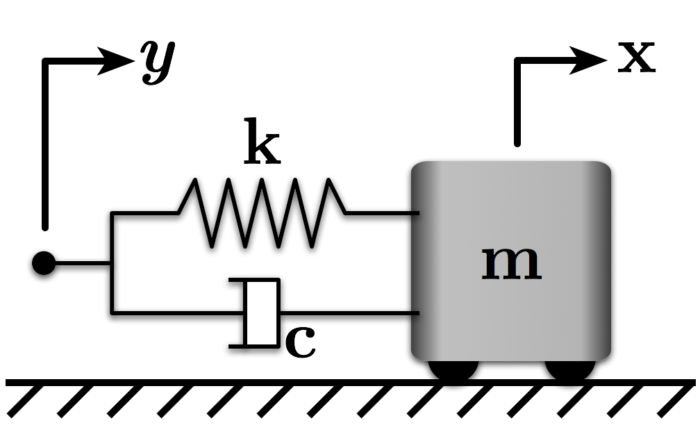
Figure 1: A Mass-Spring-Damper System
This notebook simluates a step response of a simple mass-spring-damper system like the one shown in Figure 1. We will also be using some functions from the Python Control Systems Toolbox.
The equation of motion for the system is:
$ \quad m \ddot{x} + c \dot{x} + kx = c \dot{y} + ky $
We could also write this equation in terms of the damping ratio, $\zeta$, and natural frequency, $\omega_n$.
$ \quad \ddot{x} + 2\zeta\omega_n\dot{x} + \omega_n^2x = 2\zeta\omega_n \dot{y} + \omega_n^2 y$
For information on how to obtain this equation, you can see the lectures at the class website.
We'll start by using the solution to the differential equation that we developed in class to plot the response. The solution for the underdamped case is:
$ \quad x(t) = c + e^{-\zeta\omega_nt}\left(-c \cos{\omega_d t} - \frac{\zeta c}{\sqrt{1-\zeta^2}} \sin{\omega_d t}\right) $
where $c$ is the desired step size, and $\omega_d = \omega_n \sqrt{1 - \zeta^2}$ is the damped natural frequency.
import numpy as np # Grab all of the NumPy functions with nickname np
# We want our plots to be displayed inline, not in a separate window
%matplotlib inline

import matplotlib.pyplot as plt
# Define the System Parameters
m = 1.0                 # kg
k = (2.0*np.pi)**2      # N/m (Selected to give an undamped natrual frequency of 1Hz)
wn = np.sqrt(k/m)       # Natural Frequency (rad/s)

z = 0.2                 # Define a desired damping ratio
c = 2*z*wn*m            # calculate the damping coeff. to create it (N/(m/s))

wd = wn*np.sqrt(1-z**2) # Damped natural frequency (rad/s)
# Define the time array
t = np.linspace(0, 3, 301) # 0-3s with 301 points in between

# Define the step input (We're using y_step, because we've already defined c as our damping coeff.)
y_step = 1.0

# Define x(t)
# In this case, we're specifying that the step input occurs at t = 0
x = y_step + np.exp(-z*wn*t)*(-y_step*np.cos(wd*t) + (z*y_step)/(np.sqrt(1-z**2)) * np.sin(wd*t))
# Set the plot size - 3x2 aspect ratio is best
fig = plt.figure(figsize=(6, 4))
ax = plt.gca()
plt.subplots_adjust(bottom=0.17, left=0.17, top=0.96, right=0.96)

# Change the axis units to serif
plt.setp(ax.get_ymajorticklabels(), family='serif', fontsize=18)
plt.setp(ax.get_xmajorticklabels(), family='serif', fontsize=18)

ax.spines['right'].set_color('none')
ax.spines['top'].set_color('none')

ax.xaxis.set_ticks_position('bottom')
ax.yaxis.set_ticks_position('left')

# Turn on the plot grid and set appropriate linestyle and color
ax.grid(True,linestyle=':', color='0.75')
ax.set_axisbelow(True)

# Define the X and Y axis labels
plt.xlabel('Time (s)', family='serif', fontsize=22, weight='bold', labelpad=5)
plt.ylabel('Position (m)', family='serif', fontsize=22, weight='bold', labelpad=10)

plt.plot([t[0], t[-1]], [y_step, y_step], linewidth=2, linestyle='--', label=r'Step Input')
plt.plot(t, x, linewidth=2, linestyle='-', label=r'Response')

# uncomment below and set limits if needed
# plt.xlim(0, 5)
# plt.ylim(0, 10)

# Create the legend, then fix the fontsize
leg = plt.legend(loc='upper right', ncol = 1, fancybox=True)
ltext  = leg.get_texts()
plt.setp(ltext, family='serif', fontsize=20)

# Adjust the page layout filling the page using the new tight_layout command
plt.tight_layout(pad=0.5)

# Uncommetn to save the figure as a high-res pdf in the current folder
# It's saved at the original 6x4 size
plt.savefig('Step_Response.pdf')

fig.set_size_inches(9, 6) # Resize the figure for better display in the notebook

Using the Control System Toolbox
We can also simluate responses using the Python Control Systems Library. To do so, we'll use the transfer function form of the equations of motion. If you've had controls, you probably spent a lot of time working with transfer functions. If not, we'll learn more about them later. For now, just think of a transfer function as an experssion of how the input is "transferred" to the output.
# import the control system toolbox
import control
# Define the system to use in simulation - in transfer function form here
num = [2.0*z*wn, wn**2]
den = [1.0, 2.0*z*wn, wn**2]

sys = control.tf(num,den)
# Form the step input in desired position, yd, starting the step at t=0.0s
yd = np.ones_like(t)              # This is an array of all ones, with the same size as t
# Define the initial conditions x_dot(0) = 0, x(0) = 0
x0 = [0.,0.]

# run the simulation - utilize the built-in initial condition response function
[T, yout, x_out] = control.forced_response(sys, t, yd, x0)
Now, let's plot this version of the solution. It should look the same as the function-based version.
# Set the plot size - 3x2 aspect ratio is best
fig = plt.figure(figsize=(6, 4))
ax = plt.gca()
plt.subplots_adjust(bottom=0.17, left=0.17, top=0.96, right=0.96)

# Change the axis units to serif
plt.setp(ax.get_ymajorticklabels(), family='serif', fontsize=18)
plt.setp(ax.get_xmajorticklabels(), family='serif', fontsize=18)

ax.spines['right'].set_color('none')
ax.spines['top'].set_color('none')

ax.xaxis.set_ticks_position('bottom')
ax.yaxis.set_ticks_position('left')

# Turn on the plot grid and set appropriate linestyle and color
ax.grid(True,linestyle=':', color='0.75')
ax.set_axisbelow(True)

# Define the X and Y axis labels
plt.xlabel('Time (s)', family='serif', fontsize=22, weight='bold', labelpad=5)
plt.ylabel('Position (m)', family='serif', fontsize=22, weight='bold', labelpad=10)

plt.plot(t, yd, linewidth=2, linestyle='--', label=r'Step Input')
plt.plot(t, yout, linewidth=2, linestyle='-', label=r'Response')

# uncomment below and set limits if needed
# plt.xlim(0, 5)
# plt.ylim(0, 10)

# Create the legend, then fix the fontsize
leg = plt.legend(loc='upper right', ncol = 1, fancybox=True)
ltext  = leg.get_texts()
plt.setp(ltext, family='serif', fontsize=20)

# Adjust the page layout filling the page using the new tight_layout command
plt.tight_layout(pad=0.5)

# Uncommetn to save the figure as a high-res pdf in the current folder
# It's saved at the original 6x4 size
# plt.savefig('plot_filename.pdf')

fig.set_size_inches(9, 6) # Resize the figure for better display in the notebook

Licenses
Code is licensed under a 3-clause BSD style license. See the licenses/LICENSE.md file.
Other content is provided under a Creative Commons Attribution-NonCommercial 4.0 International License, CC-BY-NC 4.0.
# This cell will just improve the styling of the notebook
# You can ignore it, if you are okay with the default sytling
from IPython.core.display import HTML
import urllib.request
response = urllib.request.urlopen("https://cl.ly/1B1y452Z1d35")
HTML(response.read().decode("utf-8"))