Free Vibration of a Mass-Spring-Damper System
MCHE 485: Mechanical Vibrations
Dr. Joshua Vaughan
joshua.vaughan@louisiana.edu
http://www.ucs.louisiana.edu/~jev9637/
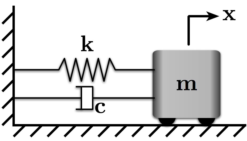
Figure 1: A Mass-Spring-Damper System
This notebook simulates the free vibration of a simple mass-spring-damper system like the one shown in Figure 1. More specifically, we'll look at how system response to non-zero initial conditions.
The equation of motion for the system is:
$ \quad m \ddot{x} + c \dot{x} + kx = 0 $
We could also write this equation in terms of the damping ratio, $\zeta$, and natural frequency $\omega_n$.
$ \quad \ddot{x} + 2\zeta\omega_n\dot{x} + \omega_n^2x = 0$
For information on how to obtain this equation, you can see the lectures at the class website.
We'll use the solution to the differential equation that we developed in class to plot the response. The solution for the underdamped case is:
$ \quad x(t) = e^{-\zeta\omega_nt}\left(a_1 e^{i \omega_d t} + a_2 e ^{-i \omega_d t}\right) $
or
$ \quad x(t) = e^{-\zeta\omega_nt}\left(b_1 \cos{\omega_d t} + b_2 \sin{\omega_d t}\right) $
To use this equation, we need to solve for $a_1$ and $a_2$ or $b_1$ and $b_2$ using the initial conditions. Here, let's use the sin/cosine form. Solving the equation for generic intial velocity, $\dot{x} = v_0$, and a generic initial displacement, $x = x_0$, we find:
$ \quad x(t) = e^{-\zeta\omega_nt}\left(x_0 \cos{\omega_d t} + \frac{\zeta \omega_n x_0 + v_0}{\omega_d} \sin{\omega_d t}\right) $
import numpy as np # Grab all of the NumPy functions with nickname np
%matplotlib inline

# Import the plotting functions
import matplotlib.pyplot as plt
# Define the System Parameters
m = 1.0                   # kg
k = (2.0 * np.pi)**2.     # N/m (Selected to give an undamped natrual frequency of 1Hz)
wn = np.sqrt(k/m)         # Natural Frequency (rad/s)

z = 0.1                   # Define a desired damping ratio
c = 2*z*wn*m              # calculate the damping coeff. to create it (N/(m/s))

wd = wn*np.sqrt(1 - z**2) # Damped natural frequency (rad/s)
# Set up simulation parameters
t = np.linspace(0, 5, 501)          # Time for simulation, 0-5s with 501 points in-between

# Define the initial conditions x(0) = 1 and x_dot(0) = 0
x0 = np.array([-1.0, 0.0])
# Define x(t)
x = np.exp(-z*wn*t)*(x0[0]*np.cos(wd*t) + (z*wn*x0[0] + x0[1])/wd * np.sin(wd*t))
# # Make the figure pretty, then plot the results
# #   "pretty" parameters selected based on pdf output, not screen output
# #   Many of these setting could also be made default by the .matplotlibrc file

# Set the plot size - 3x2 aspect ratio is best
fig = plt.figure(figsize=(6, 4))
ax = plt.gca()
plt.subplots_adjust(bottom=0.17, left=0.17, top=0.96, right=0.96)

# Change the axis units to serif
plt.setp(ax.get_ymajorticklabels(),family='serif',fontsize=18)
plt.setp(ax.get_xmajorticklabels(),family='serif',fontsize=18)

ax.spines['right'].set_color('none')
ax.spines['top'].set_color('none')

ax.xaxis.set_ticks_position('bottom')
ax.yaxis.set_ticks_position('left')

# Turn on the plot grid and set appropriate linestyle and color
ax.grid(True,linestyle=':',color='0.75')
ax.set_axisbelow(True)

# Define the X and Y axis labels
plt.xlabel('Time (s)', family='serif', fontsize=22, weight='bold', labelpad=5)
plt.ylabel('Position', family='serif', fontsize=22, weight='bold', labelpad=10)


amp = np.sqrt(x0[0]**2 + ((z*wn*x0[0] + x0[1])/wd)**2)
decay_env = amp * np.exp(-z*wn*t)

# plot the decay envelope
plt.plot(t, decay_env, linewidth=1.0, linestyle = '--', color = "#377eb8")
plt.plot(t, -decay_env, linewidth=1.0, linestyle = '--', color = "#377eb8")

plt.plot(t, x, linewidth=2, linestyle = '-', label=r'Response')

# uncomment below and set limits if needed
# xlim(0,5)
# ylim(0,10)

plt.yticks([-1.5, -1, -0.5, 0, 0.5, 1, 1.5], ['', r'$-x_0$', '', '0', '', r'$x_0$', ''])

plt.annotate('Exponential Decay Envelope',
         xy=(t[int(len(t)/3)],decay_env[int(len(t)/3)]), xycoords='data',
         xytext=(+10, +30), textcoords='offset points', fontsize=18,
         arrowprops=dict(arrowstyle="simple, head_width = 0.35, tail_width=0.05", connectionstyle="arc3, rad=.2", color="#377eb8"), color = "#377eb8")


# # Create the legend, then fix the fontsize
# leg = plt.legend(loc='upper right', fancybox=True)
# ltext  = leg.get_texts()
# plt.setp(ltext,family='serif',fontsize=18)

# Adjust the page layout filling the page using the new tight_layout command
plt.tight_layout(pad = 0.5)

# save the figure as a high-res pdf in the current folder
# It's saved at the original 6x4 size
# plt.savefig('MCHE485_FreeVibrationWithDamping.pdf')

fig.set_size_inches(9, 6) # Resize the figure for better display in the notebook

Licenses
Code is licensed under a 3-clause BSD style license. See the licenses/LICENSE.md file.
Other content is provided under a Creative Commons Attribution-NonCommercial 4.0 International License, CC-BY-NC 4.0.
# This cell will just improve the styling of the notebook
# You can ignore it, if you are okay with the default sytling
from IPython.core.display import HTML
import urllib.request
response = urllib.request.urlopen("https://cl.ly/1B1y452Z1d35")
HTML(response.read().decode("utf-8"))