Vibration Absorbers
(without damping)
MCHE 485: Mechanical Vibrations
Dr. Joshua Vaughan
joshua.vaughan@louisiana.edu
http://www.ucs.louisiana.edu/~jev9637/
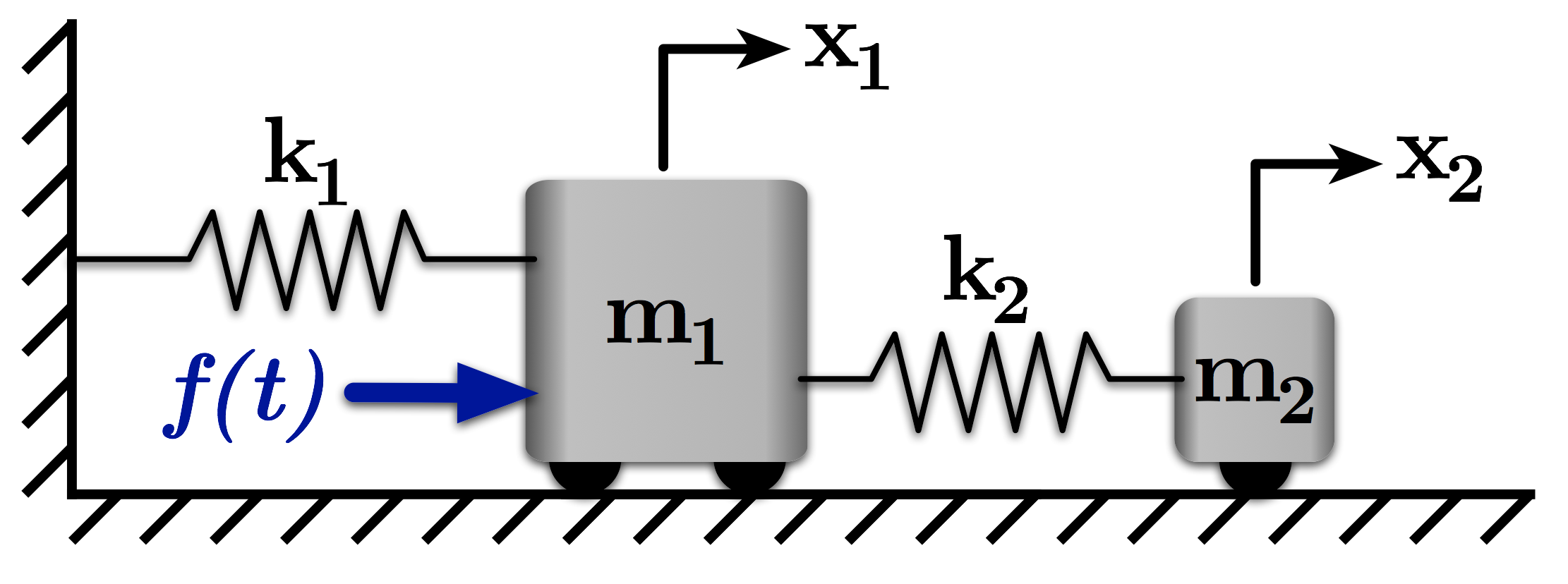
Figure 1: An Undamped Vibration Absorber System
This notebook demonstrates the analysis of a vibration absorber system like the one shown in Figure 1. The $m_2$ subsystem has been added to the system with hopes of limiting the vibration of $m_1$. For this system, to limit the vibration of $m_1$, the second mass, $m_2$, and second spring, $k_2$, must be chosen such that:
$ \quad \frac{k_2}{m_2} = \frac{k_1}{m_2} $
Let's analyze the responses of $m_1$ and $m_2$ when this condition holds. The equations of motion for the system are:
$ \quad m_1 \ddot{x}_1 + (k_1+k_2)x_1 - k_2 x_2 = f $
$ \quad m_2 \ddot{x}_2 -k_2 x_1 + k_2x_2 = 0 $
We could also write this equation in matrix form:
$ \quad \begin{bmatrix}m_1 & 0 \\ 0 & m_2\end{bmatrix}\begin{bmatrix}\ddot{x}_1 \\ \ddot{x}_2\end{bmatrix} + \begin{bmatrix}k_1 + k_2 & -k_2 \\ -k_2 & \hphantom{-}k_2\end{bmatrix}\begin{bmatrix}x_1 \\ x_2\end{bmatrix} = \begin{bmatrix}f \\ 0\end{bmatrix}$
Define
$ \quad M = \begin{bmatrix}m_1 & 0 \\ 0 & m_2\end{bmatrix} $
and
$ \quad K = \begin{bmatrix}k_1 + k_2 & -k_2 \\ -k_2 & \hphantom{-}k_2\end{bmatrix} $.
Using $M$ and $K$, we want to solve:
$ \quad \left[K - \omega^2 M\right]\bar{X} = \bar{F} $
for $\bar{X}$. To do so, we need to take the inverse of $\left[K - \omega^2 M\right]$.
$ \quad \bar{X} = \left[K - \omega^2 M\right]^{-1}\bar{F} $
For information on how to obtain these equations, you can see the lectures at the class website.
We'll use the numpy tools to solve this problem and examine the response of this vibration absorber system.
import numpy as np

# We'll use the scipy version of the linear algebra
from scipy import linalg

# Import the ODE solver for our time response analysis
from scipy.integrate import odeint
# We want our plots to be displayed inline, not in a separate window
%matplotlib inline

# Import the plotting functions
import matplotlib.pyplot as plt
# Define the matrices - We'll use the values from the book example
m1 = 100.0
m2 = 10.0

k1 = 900.0
k2 = 90.0

M = np.array([[m1, 0],
                [0,  m2]])

K = np.array([[k1 + k2, -k2],
                [-k2,      k2]])
F1 = 1.0
F2 = 0.0

F = [F1, F2]

w = np.linspace(0,6,1200)
X = np.zeros((len(w),2))

# This is (K-w^2 M)^-1 * (w^2*F)
for ii, freq in enumerate(w):
    X[ii,:] = np.dot(linalg.inv(K - freq**2 * M), F)

# Let's mask the discontinuity, so it isn't plotted
pos = np.where(np.abs(X[:,0]) >= 0.25)
X[pos,:] = np.nan
w[pos] = np.nan
# Set the plot size - 3x2 aspect ratio is best
fig = plt.figure(figsize=(6,4))
ax = plt.gca()
plt.subplots_adjust(bottom=0.17,left=0.17,top=0.96,right=0.96)

# Change the axis units to CMU Serif
plt.setp(ax.get_ymajorticklabels(),family='serif',fontsize=18)
plt.setp(ax.get_xmajorticklabels(),family='serif',fontsize=18)

ax.spines['right'].set_color('none')
ax.spines['top'].set_color('none')

ax.xaxis.set_ticks_position('bottom')
ax.yaxis.set_ticks_position('left')

# Turn on the plot grid and set appropriate linestyle and color
ax.grid(True,linestyle=':',color='0.75')
ax.set_axisbelow(True)

# Define the X and Y axis labels
plt.xlabel('Frequency (rad/s)',family='serif',fontsize=22,weight='bold',labelpad=5)
plt.ylabel('Amplitude',family='serif',fontsize=22,weight='bold',labelpad=10)

plt.plot(w,X[:,0],linewidth=2,label=r'$\bar{x}_1$')
plt.plot(w,X[:,1],linewidth=2,linestyle="--",label=r'$\bar{x}_2$')

# uncomment below and set limits if needed
plt.xlim(1.5,4.5)
plt.ylim(-0.11,0.10)

# Create the legend, then fix the fontsize
leg = plt.legend(loc='upper right', fancybox=True)
ltext  = leg.get_texts()
plt.setp(ltext,family='serif',fontsize=16)

# Adjust the page layout filling the page using the new tight_layout command
plt.tight_layout(pad=0.5)

# save the figure as a high-res pdf in the current folder
# plt.savefig('Vibration_Absorber.pdf')

fig.set_size_inches(9,6) # Resize the figure for better display in the notebook

We could also plot the magnitude of the response
# Plot the magnitude of the response

# Set the plot size - 3x2 aspect ratio is best
fig = plt.figure(figsize=(6,4))
ax = plt.gca()
plt.subplots_adjust(bottom=0.17,left=0.17,top=0.96,right=0.96)

# Change the axis units to CMU Serif
plt.setp(ax.get_ymajorticklabels(),family='serif',fontsize=18)
plt.setp(ax.get_xmajorticklabels(),family='serif',fontsize=18)

ax.spines['right'].set_color('none')
ax.spines['top'].set_color('none')

ax.xaxis.set_ticks_position('bottom')
ax.yaxis.set_ticks_position('left')

# Turn on the plot grid and set appropriate linestyle and color
ax.grid(True,linestyle=':',color='0.75')
ax.set_axisbelow(True)

# Define the X and Y axis labels
plt.xlabel('Frequency (rad/s)',family='serif',fontsize=22,weight='bold',labelpad=5)
plt.ylabel('Magnitude',family='serif',fontsize=22,weight='bold',labelpad=10)

plt.plot(w,np.abs(X[:,0]),linewidth=2,label=r'$|\bar{x}_1|$')
plt.plot(w,np.abs(X[:,1]),linewidth=2,linestyle="--",label=r'$|\bar{x}_2|$')

# uncomment below and set limits if needed
plt.xlim(1.4,4.5)
plt.ylim(-0.01,0.1)

# Create the legend, then fix the fontsize
leg = plt.legend(loc='upper right', fancybox=True)
ltext  = leg.get_texts()
plt.setp(ltext,family='serif',fontsize=16)

# Adjust the page layout filling the page using the new tight_layout command
plt.tight_layout(pad=0.5)

# save the figure as a high-res pdf in the current folder
# plt.savefig('Vibration_Absorber_Magnitude.pdf')

fig.set_size_inches(9,6) # Resize the figure for better display in the notebook

Now, let's look at using a smaller $m_2$ and $k_2$.
# Redefine the matrices with the new parameters
m1 = 100.0
m2 = 3.0

k1 = 900.0
k2 = 27.0

M = np.asarray([[m1, 0],
                [0,  m2]])

K = np.asarray([[k1 + k2, -k2],
                [-k2,      k2]])

F1 = 1.0
F2 = 0.0

F = [F1,F2]

w = np.linspace(0,6,1200)
X = np.zeros((len(w),2))

for ii, freq in enumerate(w):
	X[ii,:] = np.dot(linalg.inv(K - freq**2 * M), F)

# Let's mask the discontinuity, so it isn't plotted
pos = np.where(np.abs(X[:,0]) >= 0.25)
X[pos,:] = np.nan
w[pos] = np.nan


# Set the plot size - 3x2 aspect ratio is best
fig = plt.figure(figsize=(6,4))
ax = plt.gca()
plt.subplots_adjust(bottom=0.17,left=0.17,top=0.96,right=0.96)

# Change the axis units to CMU Serif
plt.setp(ax.get_ymajorticklabels(),family='serif',fontsize=18)
plt.setp(ax.get_xmajorticklabels(),family='serif',fontsize=18)

ax.spines['right'].set_color('none')
ax.spines['top'].set_color('none')

ax.xaxis.set_ticks_position('bottom')
ax.yaxis.set_ticks_position('left')

# Turn on the plot grid and set appropriate linestyle and color
ax.grid(True,linestyle=':',color='0.75')
ax.set_axisbelow(True)

# Define the X and Y axis labels
plt.xlabel('Frequency (rad/s)',family='serif',fontsize=22,weight='bold',labelpad=5)
plt.ylabel('Amplitude',family='serif',fontsize=22,weight='bold',labelpad=10)

plt.plot(w,X[:,0],linewidth=2,label=r'$\bar{x}_1$')
plt.plot(w,X[:,1],linewidth=2,linestyle="--",label=r'$\bar{x}_2$')

# uncomment below and set limits if needed
plt.xlim(1.5,4.5)
plt.ylim(-0.11,0.10)

# Create the legend, then fix the fontsize
leg = plt.legend(loc='upper right', fancybox=True)
ltext  = leg.get_texts()
plt.setp(ltext,family='serif',fontsize=16)

# Adjust the page layout filling the page using the new tight_layout command
plt.tight_layout(pad=0.5)

# save the figure as a high-res pdf in the current folder
# plt.savefig('Vibration_Absorber_SmallerM2K2.pdf')

fig.set_size_inches(9,6) # Resize the figure for better display in the notebook

Notice that the two natural frequencies are closer together than the previous case. This leads to a smaller range over which there is low vibration in $x_1$.
The amplitude of $x_2$ is also increased from the previous case.
We could again plot the magnitude of the response.
# Plot the magnitude of the response

# Set the plot size - 3x2 aspect ratio is best
fig = plt.figure(figsize=(6,4))
ax = plt.gca()
plt.subplots_adjust(bottom=0.17,left=0.17,top=0.96,right=0.96)

# Change the axis units to CMU Serif
plt.setp(ax.get_ymajorticklabels(),family='serif',fontsize=18)
plt.setp(ax.get_xmajorticklabels(),family='serif',fontsize=18)

ax.spines['right'].set_color('none')
ax.spines['top'].set_color('none')

ax.xaxis.set_ticks_position('bottom')
ax.yaxis.set_ticks_position('left')

# Turn on the plot grid and set appropriate linestyle and color
ax.grid(True,linestyle=':',color='0.75')
ax.set_axisbelow(True)

# Define the X and Y axis labels
plt.xlabel('Frequency (rad/s)',family='serif',fontsize=22,weight='bold',labelpad=5)
plt.ylabel('Magnitude',family='serif',fontsize=22,weight='bold',labelpad=10)

plt.plot(w,np.abs(X[:,0]),linewidth=2,label=r'$|\bar{x}_1|$')
plt.plot(w,np.abs(X[:,1]),linewidth=2,linestyle="--",label=r'$|\bar{x}_2|$')

# uncomment below and set limits if needed
plt.xlim(1.4,4.5)
plt.ylim(-0.01,0.1)

# Create the legend, then fix the fontsize
leg = plt.legend(loc='upper right', fancybox=True)
ltext  = leg.get_texts()
plt.setp(ltext,family='serif',fontsize=16)

# Adjust the page layout filling the page using the new tight_layout command
plt.tight_layout(pad=0.5)

# save the figure as a high-res pdf in the current folder
# plt.savefig('Vibration_Absorber_Magnitude.pdf')

fig.set_size_inches(9,6) # Resize the figure for better display in the notebook

Time Response
Let's take a look at the time response to confirm this phenomenon. To do so, we'll have to represent our equations of motion as a system of first order ODEs, rather than two second-order ODEs. This is the beginning of putting the equations into state space form.
Define a state vector $\mathbf{w} = \left[x \quad \dot{x_1} \quad x_2 \quad \dot{x_2}\right]^T $
Note: We'll most often see the state space form writen as:
$ \quad \dot{w} = Aw + Bu $
where $x$ is the state vector, $A$ is the state transition matrix, $B$ is the input matrix, and $u$ is the input. We'll use w here and in the code to avoid confusion with our state $x$, the position of $m_1$.
To begin, let's write the two equations of motion as:
$ \quad \ddot{x}_1 = \frac{1}{m_1} \left(-(k_1 + k_2)x_1 + k_2 x_2 + f \right)$
$ \quad \ddot{x}_2 = \frac{1}{m_2} \left(k_2 x_1 - k_2 x_2 \right)$
After some algebra and using the state vector defined above, we can write our equations of motion as:
$ \quad \dot{\mathbf{w}} = \begin{bmatrix}0 & 1 & 0 & 0\\ -\frac{k_1 + k_2}{m_1} & 0 & \frac{k_2}{m_1} & 0 \\ 0 & 0 & 0 & 1 \\ \frac{k_2}{m_2} & 0 & -\frac{k_2}{m_2} & 0 \end{bmatrix}\mathbf{w} + \begin{bmatrix}0 \\ \frac{1}{m_1} \\ 0 \\ 0 \end{bmatrix} f $
Now, let's write this in a way that our ODE solver can use it.
# Define the equations of motion

# Define the system as a series of 1st order ODEs (beginnings of state-space form)
def eq_of_motion(w, t, p):
    """
    Defines the differential equations for the coupled spring-mass system.

    Arguments:
        w :  vector of the state variables:
                  w = [x1, x1_dot, x2, x2_dot]
        t :  time
        p :  vector of the parameters:
                  p = [m1, m2, k1, k2, wf]
    """

    x1, x1_dot, x2, x2_dot = w
    m1, m2, k1, k2, wf = p

    # Create sysODE = (x1', x1_dot', x2', x2_dot')
    sysODE = [x1_dot,
             (-(k1 + k2) * x1 + k2 * x2 + f(t, p)) / m1,
             x2_dot,
             (k2 * x1 - k2 * x2) / m2]

    return sysODE


# Define the forcing function
def f(t, p):
    """
    Defines the forcing function

    Arguments:
        t : time
        p :  vector of the parameters:
             p = [m1, m2, k1, k2, wf]

    Returns:
        f : forcing function at current timestep
    """

    m1, m2, k1, k2, wf = p

    # Uncomment below for no force input - use for initial condition response
    #f = 0.0

    # Uncomment below for sinusoidal forcing input at frequency wf rad/s
    f = 10 * np.sin(wf * t)

    return f
# Set up simulation parameters

# ODE solver parameters
abserr = 1.0e-9
relerr = 1.0e-9
max_step = 0.01
stoptime = 100.0
numpoints = 10001

# Create the time samples for the output of the ODE solver
t = np.linspace(0.0, stoptime, numpoints)

# Initial conditions
x1_init = 0.0                    # initial position
x1_dot_init = 0.0                # initial velocity
x2_init = 0.0                    # initial angle
x2_dot_init = 0.0                # initial angular velocity

wf = np.sqrt(k1 / m1)             # forcing function frequency

# Pack the parameters and initial conditions into arrays
p = [m1, m2, k1, k2, wf]
x0 = [x1_init, x1_dot_init, x2_init, x2_dot_init]
# Call the ODE solver.
resp = odeint(eq_of_motion, x0, t, args=(p,), atol=abserr, rtol=relerr,  hmax=max_step)
# Set the plot size - 3x2 aspect ratio is best
fig = plt.figure(figsize=(6,4))
ax = plt.gca()
plt.subplots_adjust(bottom=0.17,left=0.17,top=0.96,right=0.96)

# Change the axis units to serif
plt.setp(ax.get_ymajorticklabels(),family='serif',fontsize=18)
plt.setp(ax.get_xmajorticklabels(),family='serif',fontsize=18)

ax.spines['right'].set_color('none')
ax.spines['top'].set_color('none')

ax.xaxis.set_ticks_position('bottom')
ax.yaxis.set_ticks_position('left')

# Turn on the plot grid and set appropriate linestyle and color
ax.grid(True,linestyle=':',color='0.75')
ax.set_axisbelow(True)

# Define the X and Y axis labels
plt.xlabel('Time (s)',family='serif',fontsize=22,weight='bold',labelpad=5)
plt.ylabel('Position (m)',family='serif',fontsize=22,weight='bold',labelpad=10)

plt.plot(t, resp[:,0],linewidth=2,label=r'$x_1$')
plt.plot(t, resp[:,2],linewidth=2,linestyle="--",label=r'$x_2$')

# uncomment below and set limits if needed
# plt.xlim(0,5)
plt.ylim(-1,1)


# Create the legend, then fix the fontsize
leg = plt.legend(loc='upper right', ncol=2, fancybox=True)
ltext  = leg.get_texts()
plt.setp(ltext,family='serif',fontsize=18)

# Adjust the page layout filling the page using the new tight_layout command
plt.tight_layout(pad=0.5)

# save the figure as a high-res pdf in the current folder
# It's saved at the original 6x4 size
# plt.savefig('Undamped_VibAbsorber_TimeResponse.pdf')

fig.set_size_inches(9,6) # Resize the figure for better display in the notebook

Wait... It's NOT a Vibration Absorber?!?!?
Remember that our frequency domain analysis assumes steady-state responses. In this simulation, that is not the case. We have some transient oscillation that occurs as our system transitions from rest to being forced according to $f(t)$. If the system has no damping, like this one, then this transient response never decays.
Notice, however, that the ampliude of $x(t)$ is bounded. It would not be without the attached mass, $m_2$. We're forcing at the original $m_1,k_1$ subystem's natural frequency, so it would grow to inifinity.
Licenses
Code is licensed under a 3-clause BSD style license. See the licenses/LICENSE.md file.
Other content is provided under a Creative Commons Attribution-NonCommercial 4.0 International License, CC-BY-NC 4.0.
# This cell will just improve the styling of the notebook
# You can ignore it, if you are okay with the default sytling
from IPython.core.display import HTML
import urllib.request
response = urllib.request.urlopen("https://cl.ly/1B1y452Z1d35")
HTML(response.read().decode("utf-8"))