Multi-DOF Example
MCHE 485: Mechanical Vibrations
Dr. Joshua Vaughan
joshua.vaughan@louisiana.edu
http://www.ucs.louisiana.edu/~jev9637/
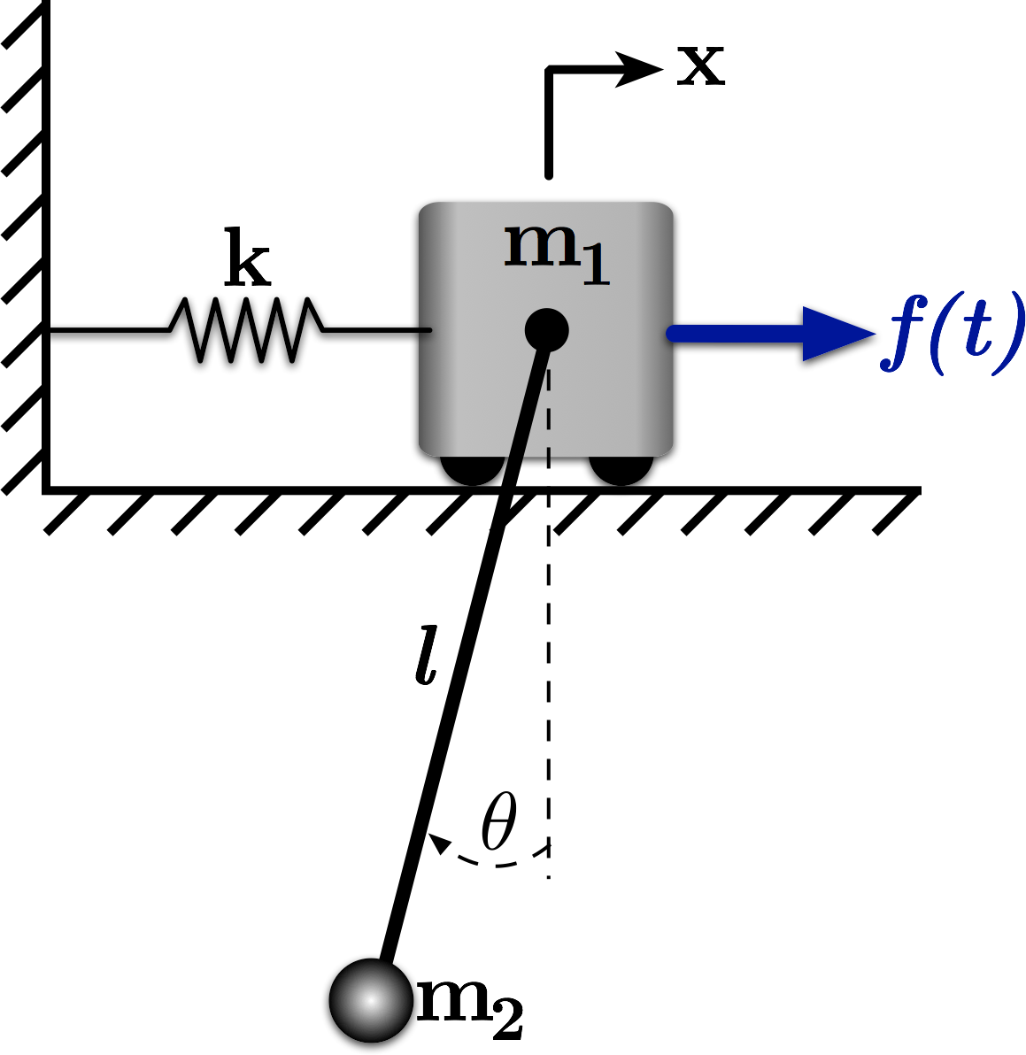
Figure 1: An Undamped Multi-Degree-of-Freedom System
This notebook demonstrates the analysis of the system shown in Figure 1. Mass $m_1$ is attached to ground via a spring and constrained to move horizontally. Its horizontal motion from equilibrium is described by $x$. Mass $m_2$ is suspended from the center of $m_1$ via a massless, inextensible, inflexible cable of length $l$. The angle of this cable from horizontal is described by $\theta$. The equations of motion for the system are:
$ \quad \left(m_1 + m_2\right) \ddot{x} - m_2 l \ddot{\theta} + k x = f $
$ \quad -m_2 l \ddot{x} + m_2 l^2 \ddot{\theta} + m_2 g l \theta = 0 $
We could also write this equation in matrix form:
$ \quad \begin{bmatrix}m_1 + m_2 & -m_2 l \\ -m_2 l & \hphantom{-}m_2 l^2\end{bmatrix}\begin{bmatrix}\ddot{x} \\ \ddot{\theta}\end{bmatrix} + \begin{bmatrix}k & 0 \\ 0 & m_2 g l\end{bmatrix}\begin{bmatrix}x \\ \theta\end{bmatrix} = \begin{bmatrix}f \\ 0\end{bmatrix}$
Define
$ \quad M = \begin{bmatrix}m_1 + m_2 & -m_2 l \\ -m_2 l & \hphantom{-}m_2 l^2\end{bmatrix} $
and
$ \quad K = \begin{bmatrix}k & 0 \\ 0 & m_2 g l\end{bmatrix} $.
For information on how to obtain these equations, you can see the lectures at the class website.
We'll use the NumPy and SciPy tools to solve this problem and examine the response of this system.
import numpy as np

# We'll use the scipy version of the linear algebra
from scipy import linalg

# We'll also use the ode solver to plot the time response
from scipy.integrate import odeint
# We want our plots to be displayed inline, not in a separate window
%matplotlib inline

# Import the plotting functions
import matplotlib.pyplot as plt
# Define the matrices
m1 = 10.0
m2 = 1.0
g = 9.81
k = 4 * np.pi**2
l = (m1 * g) / k
c = 2.0

M = np.asarray([[m1 + m2, -m2 * l],
                [-m2 * l,  m2 * l**2]])

K = np.asarray([[k, 0],
                [0, m2 * g * l]])
The Eigenvalue/Eigenvector Problem
Let's first look at the eigenvalue/eigenvector problem in order to determine the natural frequencies and mode-shapes for this system.
Using $M$ and $K$, we want to solve:
$ \quad \left[K - \omega^2 M\right]\bar{X} = 0 $
for $\bar{X}$.
eigenvals, eigenvects = linalg.eigh(K,M)

print('\n')
print('The resulting eigenalues are {:.2f} and {:.2f}.'.format(eigenvals[0], eigenvals[1]))
print('\n')
print('So the two natrual frequencies are {:.2f}rad/s and {:.2f}rad/s.'.format(np.sqrt(eigenvals[0]), np.sqrt(eigenvals[1])))
print('\n\n')
print('The first eigenvector is {}.'.format(eigenvects[:,0]))
print('\n')
print('The second eigenvector is {}.'.format(eigenvects[:,1]))
print('\n')
The resulting eigenalues are 2.88 and 5.41.


So the two natrual frequencies are 1.70rad/s and 2.33rad/s.


The first eigenvector is [-0.20540524  0.22331464].


The second eigenvector is [ 0.24043437  0.35815608].
Forced Resposne
Now, let's look at the forced response.
Using $M$ and $K$, we want to solve:
$ \quad \left[K - \omega^2 M\right]\bar{X} = \bar{F} $
for $\bar{X}$. To do so, we need to take the inverse of $\left[K - \omega^2 M\right]$.
$ \quad \bar{X} = \left[K - \omega^2 M\right]^{-1}\bar{F} $
F1 = 1.0
F2 = 0.0

F = [F1, F2]

w = np.linspace(0,6,1200)
X = np.zeros((len(w),2))

# This is (K-w^2 M)^-1 * F
for ii, freq in enumerate(w):
    X[ii,:] = np.dot(linalg.inv(K - freq**2 * M), F)

# Let's mask the discontinuity, so it isn't plotted
pos = np.where(np.abs(X[:,0]) >= 0.5)
X[pos,:] = np.nan
w[pos] = np.nan
# Set the plot size - 3x2 aspect ratio is best
fig = plt.figure(figsize=(6,4))
ax = plt.gca()
plt.subplots_adjust(bottom=0.17,left=0.17,top=0.96,right=0.96)

# Change the axis units to CMU Serif
plt.setp(ax.get_ymajorticklabels(),family='serif',fontsize=18)
plt.setp(ax.get_xmajorticklabels(),family='serif',fontsize=18)

ax.spines['right'].set_color('none')
ax.spines['top'].set_color('none')

ax.xaxis.set_ticks_position('bottom')
ax.yaxis.set_ticks_position('left')

# Turn on the plot grid and set appropriate linestyle and color
ax.grid(True,linestyle=':',color='0.75')
ax.set_axisbelow(True)

# Define the X and Y axis labels
plt.xlabel('Frequency (rad/s)',family='serif',fontsize=22,weight='bold',labelpad=5)
plt.ylabel('Amplitude',family='serif',fontsize=22,weight='bold',labelpad=10)

plt.plot(w,X[:,0],linewidth=2,label=r'$\bar{x}$')
plt.plot(w,X[:,1],linewidth=2,linestyle="--",label=r'$\bar{\theta}$')

# uncomment below and set limits if needed
# plt.xlim(0,4.5)
plt.ylim(-0.4,0.40)

# Create the legend, then fix the fontsize
leg = plt.legend(loc='upper right', fancybox=True)
ltext  = leg.get_texts()
plt.setp(ltext,family='serif',fontsize=18)

# Adjust the page layout filling the page using the new tight_layout command
plt.tight_layout(pad=0.5)

# save the figure as a high-res pdf in the current folder
# plt.savefig('Spring_Pendulum_Example_Amp.pdf')

fig.set_size_inches(9,6) # Resize the figure for better display in the notebook

We could also plot the magnitude of the response
# Plot the magnitude of the response

# Set the plot size - 3x2 aspect ratio is best
fig = plt.figure(figsize=(6,4))
ax = plt.gca()
plt.subplots_adjust(bottom=0.17,left=0.17,top=0.96,right=0.96)

# Change the axis units to CMU Serif
plt.setp(ax.get_ymajorticklabels(),family='serif',fontsize=18)
plt.setp(ax.get_xmajorticklabels(),family='serif',fontsize=18)

ax.spines['right'].set_color('none')
ax.spines['top'].set_color('none')

ax.xaxis.set_ticks_position('bottom')
ax.yaxis.set_ticks_position('left')

# Turn on the plot grid and set appropriate linestyle and color
ax.grid(True,linestyle=':',color='0.75')
ax.set_axisbelow(True)

# Define the X and Y axis labels
plt.xlabel('Frequency (rad/s)', family='serif', fontsize=22, weight='bold', labelpad=5)
plt.ylabel('Magnitude', family='serif', fontsize=22, weight='bold', labelpad=10)

plt.plot(w, np.abs(X[:,0]), linewidth=2, label=r'$|\bar{x}|$')
plt.plot(w, np.abs(X[:,1]), linewidth=2, linestyle="--", label=r'$|\bar{\theta}|$')

# uncomment below and set limits if needed
# plt.xlim(0,4.5)
plt.ylim(-0.01, 0.3)

# Create the legend, then fix the fontsize
leg = plt.legend(loc='upper right', fancybox=True)
ltext  = leg.get_texts()
plt.setp(ltext,family='serif',fontsize=18)

# Adjust the page layout filling the page using the new tight_layout command
plt.tight_layout(pad=0.5)

# save the figure as a high-res pdf in the current folder
# plt.savefig('Spring_Pendulum_Example_Mag.pdf')

fig.set_size_inches(9,6) # Resize the figure for better display in the notebook
/Users/josh/anaconda/lib/python3.6/site-packages/ipykernel_launcher.py:26: RuntimeWarning: invalid value encountered in absolute
/Users/josh/anaconda/lib/python3.6/site-packages/ipykernel_launcher.py:27: RuntimeWarning: invalid value encountered in absolute

A Vibration Absorber!?!?!
In this case, we can see that there is some frequency that the pendulum acts as a vibration absorber for $m_1$ (i.e. The magnitude of the $x$ response, $|\bar{x}|$, goes to zero at that frequency.).
Time Response
Let's take a look at the time response to confirm this phenomenon. To do so, we'll have to represent our equations of motion as a system of first order ODEs, rather than two second-order ODEs. This is the beginning of putting the equations into state space form.
Define a state vector $\mathbf{w} = \left[x \quad \dot{x} \quad \theta \quad \dot{\theta}\right]^T $
Note: We'll most often see the state space form writen as:
$ \quad \dot{w} = Aw + Bu $
where $x$ is the state vector, $A$ is the state transition matrix, $B$ is the input matrix, and $u$ is the input. We'll use w here and in the code to avoid confusion with our state $x$, the position of $m_1$.
To begin, let's write the two equations of motion as:
$ \quad \ddot{x} = \frac{1}{m_1 + m_2} \left(m_2 l \ddot{\theta} - k x + f \right)$
$ \quad \ddot{\theta}= \frac{1}{m_2 l^2} \left(m_2 l \ddot{x} - m_2 g l \theta\right) = \frac{1}{l}\ddot{x} - \frac{g}{l}\theta $
After some algebra and using the state vector defined above, we can write our equations of motion as:
$ \quad \dot{\mathbf{w}} = \begin{bmatrix}0 & 1 & 0 & 0\\ -\frac{k}{m_1} & 0 & -\frac{m_2}{m_1}g & 0 \\ 0 & 0 & 0 & 1 \\ -\frac{k}{m 1} & 0 & -\left(\frac{m_1 + m_2}{m_1}\right)\frac{g}{l} & 0 \end{bmatrix}\mathbf{w} + \begin{bmatrix}0 \\ 1 \\ 0 \\ \frac{1}{l} \end{bmatrix} f $
Now, let's write this in a way that our ODE solver can use it.
# Define the system as a series of 1st order ODES (beginnings of state-space form)
def eq_of_motion(w, t, p):
    """
    Defines the differential equations for the coupled spring-mass system.

    Arguments:
        w :  vector of the state variables:
                  w = [x, x_dot, theta, theta_dot]
        t :  time
        p :  vector of the parameters:
                  p = [m1, m2, k, c, l, g, wf]

    Returns:
        sysODE : An list representing the system of equations of motion as 1st order ODEs
    """
    x, x_dot, theta, theta_dot = w
    m1, m2, k, c, l, g, wf = p

    # Create sysODE = (x', x_dot'):
    sysODE = [x_dot,
              -k/m1 * x - m2/m1 * g * theta + f(t,p),
              theta_dot,
              -k/(m1 * l) * x - (m1 + m2)/m1 * g/l * theta + f(t,p)/l]
    return sysODE


# Define the forcing function
def f(t,p):
    """
    Defines the forcing function

    Arguments:
        t : time
        p :  vector of the parameters:
             p = [m1, m2, k, l, g, wf]

    Returns:
        f : forcing function at current timestep
    """

    m1, m2, k, c, l, g, wf = p

    # Uncomment below for no force input - use for initial condition response
    #f = 0.0

    # Uncomment below for sinusoidal forcing input at frequency wf rad/s
    f = np.sin(wf * t)

    return f
# Set up simulation parameters

# ODE solver parameters
abserr = 1.0e-9
relerr = 1.0e-9
max_step = 0.01
stoptime = 100.0
numpoints = 10001

# Create the time samples for the output of the ODE solver
t = np.linspace(0.,stoptime,numpoints)

# Initial conditions
x_init = 0.0                        # initial position
x_dot_init = 0.0                    # initial velocity
theta_init = 0.0                    # initial angle
theta_dot_init = 0.0                # initial angular velocity

wf = np.sqrt(k / m1)                  # forcing function frequency

# Pack the parameters and initial conditions into arrays
p = [m1, m2, k, c, l, g, wf]
x0 = [x_init, x_dot_init, theta_init, theta_dot_init]
# Call the ODE solver.
resp = odeint(eq_of_motion, x0, t, args=(p,), atol=abserr, rtol=relerr,  hmax=max_step)
# Make the figure pretty, then plot the results
#   "pretty" parameters selected based on pdf output, not screen output
#   Many of these setting could also be made default by the .matplotlibrc file
fig = plt.figure(figsize=(6,4))
ax = plt.gca()
plt.subplots_adjust(bottom=0.17,left=0.17,top=0.96,right=0.96)
plt.setp(ax.get_ymajorticklabels(),family='serif',fontsize=18)
plt.setp(ax.get_xmajorticklabels(),family='serif',fontsize=18)
ax.spines['right'].set_color('none')
ax.spines['top'].set_color('none')
ax.xaxis.set_ticks_position('bottom')
ax.yaxis.set_ticks_position('left')
ax.grid(True,linestyle=':',color='0.75')
ax.set_axisbelow(True)

plt.xlabel('Time (s)',family='serif',fontsize=22,weight='bold',labelpad=5)
plt.ylabel(r'Position (m \textit{or} rad)',family='serif',fontsize=22,weight='bold',labelpad=10)
# plt.ylim(-1.,1.)

# plot the response
plt.plot(t,resp[:,0], linestyle = '-', linewidth=2, label = '$x$')
plt.plot(t,resp[:,2], linestyle = '--', linewidth=2, label = r'$\theta$')

# Adjust the page layout filling the page using the new tight_layout command
plt.tight_layout(pad=0.5)

# Create the legend, then fix the fontsize
leg = plt.legend(loc='upper right', ncol = 2, fancybox=True)
ltext  = leg.get_texts()
plt.setp(ltext,family='serif',fontsize=18)

# If you want to save the figure, uncomment the commands below.
# The figure will be saved in the same directory as your IPython notebook.
# Save the figure as a high-res pdf in the current folder
# plt.savefig('Spring_Pendulum_Example_TimeResp_Undamped.pdf')

fig.set_size_inches(9,6) # Resize the figure for better display in the notebook

Wait... It's NOT a Vibration Absorber?!?!?
Remember that our frequency domain analysis assumes steady-state responses. In this simulation, that is not the case. We have some transient oscillation that occurs as our system transitions from rest to being forced according to $f(t)$. If the system has no damping, like this one, then this transient response never decays.
Notice, however, that the ampliude of $x(t)$ is bounded. It would not be without the attached pendulum. (We're forcing at the $m_1/k$ subystem's natural frequency, so it would grow to inifinity.)
Now, let's investigate how the system would behave with even a small amount of damping (which all real systems have). Let's just add a light damper between $m_1$ and ground, in parallel with the spring and of damping coefficient $c$, as shown in Figure 2.
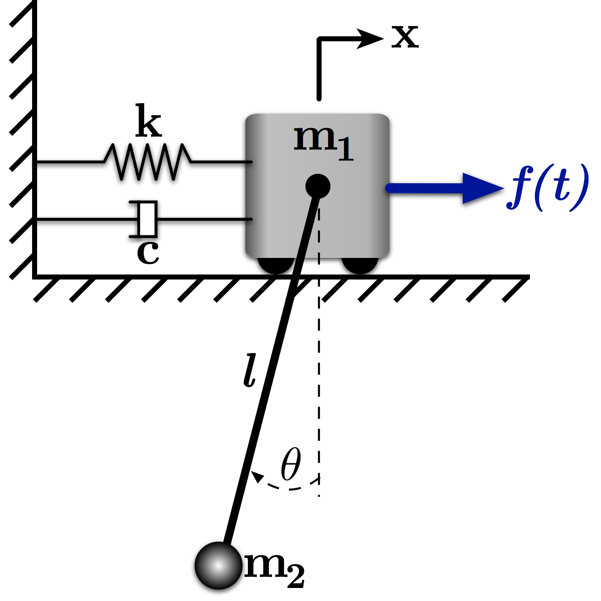
Figure 2: An Damped Multi-Degree-of-Freedom System
# Define the system as a series of 1st order ODES (beginnings of state-space form)
def eq_of_motion_damped(w, t, p):
    """
    Defines the differential equations for the coupled spring-mass system.

    Arguments:
        w :  vector of the state variables:
                  w = [x, x_dot, theta, theta_dot]
        t :  time
        p :  vector of the parameters:
                  p = [m1, m2, k, l, g, wf]

    Returns:
        sysODE : An list representing the system of equations of motion as 1st order ODEs
    """
    x, x_dot, theta, theta_dot = w
    m1, m2, k, c, l, g, wf = p

    # Create sysODE = (x', x_dot'):
    sysODE = [x_dot,
              -k/m1 * x  - c/m1 * x_dot - m2/m1 * g * theta + f(t,p),
              theta_dot,
              -k/(m1 * l) * x - c/(m1 * l) * x_dot - (m1 + m2)/m1 * g/l * theta + f(t,p)/l]
    return sysODE
# Call the ODE solver.
resp_damped = odeint(eq_of_motion_damped, x0, t, args=(p,), atol=abserr, rtol=relerr,  hmax=max_step)
# Make the figure pretty, then plot the results
#   "pretty" parameters selected based on pdf output, not screen output
#   Many of these setting could also be made default by the .matplotlibrc file
fig = plt.figure(figsize=(6,4))
ax = plt.gca()
plt.subplots_adjust(bottom=0.17,left=0.17,top=0.96,right=0.96)
plt.setp(ax.get_ymajorticklabels(),family='serif',fontsize=18)
plt.setp(ax.get_xmajorticklabels(),family='serif',fontsize=18)
ax.spines['right'].set_color('none')
ax.spines['top'].set_color('none')
ax.xaxis.set_ticks_position('bottom')
ax.yaxis.set_ticks_position('left')
ax.grid(True,linestyle=':',color='0.75')
ax.set_axisbelow(True)

plt.xlabel('Time (s)',family='serif',fontsize=22,weight='bold',labelpad=5)
plt.ylabel(r'Position (m \textit{or} rad)',family='serif',fontsize=22,weight='bold',labelpad=10)
# plt.ylim(-1.,1.)

# plot the response
plt.plot(t,resp_damped[:,0], linestyle = '-', linewidth=2, label = '$x$')
plt.plot(t,resp_damped[:,2], linestyle = '--', linewidth=2, label = r'$\theta$')

# Adjust the page layout filling the page using the new tight_layout command
plt.tight_layout(pad=0.5)

# Create the legend, then fix the fontsize
leg = plt.legend(loc='upper right', ncol = 2, fancybox=True)
ltext  = leg.get_texts()
plt.setp(ltext,family='serif',fontsize=18)

# If you want to save the figure, uncomment the commands below.
# The figure will be saved in the same directory as your IPython notebook.
# Save the figure as a high-res pdf in the current folder
# plt.savefig('Spring_Pendulum_Example_TimeResp_Damped.pdf')

fig.set_size_inches(9,6) # Resize the figure for better display in the notebook

Ahhh... Now it's a Vibration Absorber?
In this response, we can see that the damper eventually drives the transient vibration to zero, and, given enough time, the response of $x$ would approach zero as well. The peak-to-peak amplitude of the pendulum oscillation would also approach a constant value.
Licenses
Code is licensed under a 3-clause BSD style license. See the licenses/LICENSE.md file.
Other content is provided under a Creative Commons Attribution-NonCommercial 4.0 International License, CC-BY-NC 4.0.
# This cell will just improve the styling of the notebook
# You can ignore it, if you are okay with the default styling
from IPython.core.display import HTML
import urllib.request
response = urllib.request.urlopen("https://cl.ly/1B1y452Z1d35")
HTML(response.read().decode("utf-8"))