In this notebook we'll describe the basics of the Element RNN library, which is a general RNN library, and also offers implementations of LSTM and GRU recurrent networks as special cases. You should check out the documentation and examples at https://github.com/Element-Research/rnn
(P.S. The math in this notebook seems to render better in Firefox than in Chrome).
Review
Recall that a recurrent neural network maps a sequence of vectors $\mathbf{x}_1, \ldots, \mathbf{x}_n$ to a sequence of vectors $\mathbf{s}_1, \ldots, \mathbf{s}_n$ using the recurrence
\begin{align*} \mathbf{s}_{i} = R(\mathbf{x}_{i}, \mathbf{s}_{i-1}; \mathbf{\theta}), \end{align*}where $R$ is a function parameterized by $\mathbf{\theta}$, and we define $\mathbf{s}_0$ as some initial vector (such as a vector of all zeros).
N.B. For the first part of this notebook we will deal only with "acceptor" RNNs
- That is, we'll assume we only use the final state $\mathbf{s}_n$ for making predictions
- In your homework, however, you will need to implement transducer RNNs
Element RNN Basics
At the heart of the Element RNN library is the abstract class 'AbstractRecurrent', which is designed to allow calling :forward() on each element $\mathbf{x}_i$ of a sequence (in turn), with the abstract class keeping track of the $\mathbf{s}_i$ for you. Consider the following example.
require 'rnn' -- this imports 'nn' as well, and adds 'rnn' objects to the 'nn' namespace

n = 3 -- sequence length
d_in = 5 -- size of input vectors
d_hid = 5 -- size of RNN hidden state

lstm = nn.LSTM(d_in, d_hid) -- inherits from AbstractRecurrent; expects inputs in R^{d_in} and produces outputs in R^{d_hid}
data = torch.randn(n, d_in) -- a sequence of n random vectors x_1, x_2, x_3, each in R^{d_in}
outputs = torch.zeros(n, d_hid)

for i = 1, data:size(1) do
    outputs[i] = lstm:forward(data[i]) -- note that we don't need to keep track of the s_i
end

print(outputs)
 0.1089  0.0286  0.0186 -0.0631 -0.1583
 0.1212 -0.0003 -0.1499 -0.0686 -0.1137
-0.0152 -0.4429 -0.2907  0.1953  0.0102
[torch.DoubleTensor of size 3x5]
Above, the lstm is able to compute :forward() at each step by keeping track of its states internally. As we discussed in lecture, in an LSTM the states $\mathbf{s}_i$ comprise the 'hidden state' $\mathbf{h}_i$ as well as the 'cell' $\mathbf{c}_i$. In the RNN package's terminology, the $\mathbf{h}_i$ are known as 'outputs', and the $\mathbf{c}_i$ as 'cells', and these are stored internally in the nn.LSTM object, as tables:
print(lstm.outputs)
print(lstm.cells)
{
  1 : DoubleTensor - size: 5
  2 : DoubleTensor - size: 5
  3 : DoubleTensor - size: 5
}
{
  1 : DoubleTensor - size: 5
  2 : DoubleTensor - size: 5
  3 : DoubleTensor - size: 5
}
We can see that lstm.outputs are the same as the outputs tensor we stored manually
print(lstm.outputs[1])
print(lstm.outputs[2])
print(lstm.outputs[3])
 0.1089
 0.0286
 0.0186
-0.0631
-0.1583
[torch.DoubleTensor of size 5]

 0.1212
-0.0003
-0.1499
-0.0686
-0.1137
[torch.DoubleTensor of size 5]

-0.0152
-0.4429
-0.2907
 0.1953
 0.0102
[torch.DoubleTensor of size 5]
So, the first thing the RNN library gives us is implementations of many of the $R$ functions we're interested in using, such as LSTMs, and GRUs. However, it does much more!
BPTT
To do backpropagation (through time) correctly, we would technically need to loop backwards over the input sequence, as in the following pseudocode:
-- note this doesn't work! just supposed to convey how you might have to implement this...
dLdh_i = gradOutForFinalH()
dLdc_i = gradOutForFinalC()

for i = data:size(1), 1, -1 do
    dLdh_iminus1, dLdc_iminus1 = lstm:backward(data[i], {dLdh_i, dLdc_i})
    dLdh_i, dLdc_i = dLdh_iminus1, dLdc_iminus1
end
Fortunately, however, the Element RNN library can do this for us, using its nn.Sequencer objects!
Sequencers
An nn.Sequencer transforms an nn module into one that can call :forward() on an entire sequence as well as :backward() on an entire sequence, thus abstracting away the looping required for both forward propagation and backpropagation (through time).
In particular, an nn.Sequencer expects a table t_i as input, where t_i[1] $=\mathbf{x}_1$, t_i[2] $=\mathbf{x}_2$, and so on. The Sequencer outputs a table t_o, where t_o[1] $=\mathbf{h}_1$, t_o[2] $=\mathbf{h}_2$, and so on. As a warm-up, let's wrap a Linear layer with a Sequencer:
seqLin = nn.Sequencer(nn.Linear(d_in, d_hid))
t_i = torch.split(data, 1) -- make a table from our sequence of 3 vectors
t_o = seqLin:forward(t_i)
print(t_o) -- t_o gives the output of the Linear layer applied to each element in t_i
{
  1 : DoubleTensor - size: 1x5
  2 : DoubleTensor - size: 1x5
  3 : DoubleTensor - size: 1x5
}
More interestingly, we can also do this with recurrent modules, such as LSTM. Because LSTM modules (which inherit from AbstractRecurrent) maintain their previous state internally, the following correctly implements an LSTM's forward propagation over the sequence represented by t_i
seqLSTM = nn.Sequencer(nn.LSTM(d_in, d_hid))
t_o = seqLSTM:forward(t_i)
print(t_o)
{
  1 : DoubleTensor - size: 1x5
  2 : DoubleTensor - size: 1x5
  3 : DoubleTensor - size: 1x5
}
For calling :backward(), an nn.Sequencer expects gradOutput in the same shape as its input, just as every other nn module does. In this case, then, an nn.Sequencer expects gradOutput to be table with an entry for each time step. In particular, gradOutput[i] should contain:
If we're dealing with "acceptor" RNNs, which look like this:
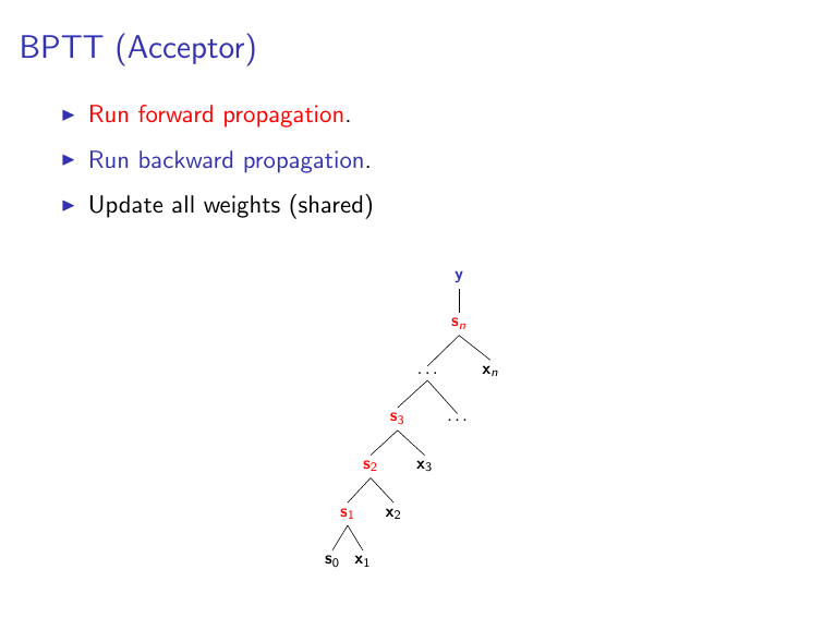
then we only generate a prediction at the $n$'th time-step (using $\mathbf{s}_n$), and there is therefore only loss at the $n$'th time-step. Accordingly, gradOutput[i] is going to be all zeros when $i < n$. This can be implemented in code as follows:
gradOutput = torch.split(torch.zeros(n, d_hid), 1) -- all zero except last time-step
-- we generally get the nonzero part of gradOutput from a criterion, so for illustration we'll use an MSECriterion
-- and some random data
mseCrit = nn.MSECriterion()
randTarget = torch.randn(t_o[n]:size())
mseCrit:forward(t_o[n], randTarget)
finalGradOut = mseCrit:backward(t_o[n], randTarget)
gradOutput[n] = finalGradOut
-- now we can BPTT with a single call!
seqLSTM:backward(t_i, gradOutput)
Avoiding Tables
Since your data will generally not be in tables (but in tensors), it's common to add additional layers to your network to map from tables to tensors and back. For instance, we can create an lstm that takes in a tensor (rather than a table), by using an nn.SplitTable
seqLSTM2 = nn.Sequential():add(nn.SplitTable(1)):add(nn.Sequencer(nn.LSTM(d_in, d_hid)))
print(seqLSTM2:forward(data))
{
  1 : DoubleTensor - size: 5
  2 : DoubleTensor - size: 5
  3 : DoubleTensor - size: 5
}
In an acceptor RNN we only care about the last state, so we can make our final layer a SelectTable (which also simplifies calling :backward(), since it implicitly passes back zeroes for all but the selected table index)
seqLSTM3 = nn.Sequential():add(nn.SplitTable(1)):add(nn.Sequencer(nn.LSTM(d_in, d_hid)))
seqLSTM3:add(nn.SelectTable(-1)) -- select the last element in the output table

print(seqLSTM3:forward(data))
gradOutFinal = gradOutput[#gradOutput] -- note that gradOutFinal is just a tensor
seqLSTM3:backward(data, gradOutFinal)
 0.0791
-0.3804
 0.1164
-0.0835
-0.0183
[torch.DoubleTensor of size 5]
If you cared about more than the last state of your LSTM, you could add an nn.JoinTable to your network after the Sequencer, which would give a tensor as output.
A More Realistic Example
To make what we've seen so far a little more concrete, let's consider training an LSTM to predict whether song lyric 5-grams from 2012 are from a timeless masterpiece or not. Here's some data:
-- our vocabulary
V = {["I"]=1, ["you"]=2, ["the"]=3, ["this"]=4, ["to"]=5, ["fire"]=6, ["Hey"]=7, ["is"]=8,
    ["just"]=9, ["zee"]=10, ["And"]=11, ["just"]=12, ["rain"]=13, ["cray"]=14, ["met"]=15, ["Set"]=16}

-- get indices of words in each 5-gram
songData = torch.LongTensor({ { V["Hey"],   V["I"],      V["just"],  V["met"],    V["you"] },
                              { V["And"],   V["this"],   V["is"],    V["cray"],   V["zee"] },
                              { V["Set"],   V["fire"],   V["to"],    V["the"],    V["rain"] } })

masterpieceOrNot = torch.Tensor({{1},   -- #carlyrae4ever
                                 {1},
                                 {0}})

print(songData)
-- we'll use a LookupTable to map word indices into vectors in R^6
vocab_size = 16
embed_dim = 6
LT = nn.LookupTable(vocab_size, embed_dim)

-- Using a Sequencer, let's make an LSTM that consumes a sequence of song-word embeddings
songLSTM = nn.Sequential()
songLSTM:add(LT) -- for a single sequence, will return a sequence-length x embedDim tensor
songLSTM:add(nn.SplitTable(1)) -- splits tensor into a sequence-length table containing vectors of size embedDim
songLSTM:add(nn.Sequencer(nn.LSTM(embed_dim, embed_dim)))
songLSTM:add(nn.SelectTable(-1)) -- selects last state of the LSTM
songLSTM:add(nn.Linear(embed_dim, 1)) -- map last state to a score for classification
songLSTM:add(nn.Sigmoid()) -- convert score to a probability
firstSongPred = songLSTM:forward(songData[1])
print(firstSongPred)
  7   1  12  15   2
 11   4   8  14  10
 16   6   5   3  13
[torch.LongTensor of size 3x5]
 0.5808
[torch.DoubleTensor of size 1]
-- we can then use a simple BCE Criterion for backprop
bceCrit = nn.BCECriterion()
loss = bceCrit:forward(firstSongPred, masterpieceOrNot[1])
dLdPred = bceCrit:backward(firstSongPred, masterpieceOrNot[1])
songLSTM:backward(songData[1], dLdPred)
Batching
In order to make RNNs fast, it is important to batch. When batching with an Element RNN, time-steps continue to be represented as indices in a table, but this time each element in the table is a matrix rather than a vector. In particular, batching occurs along the first dimension (as usual), as in the following example:
-- data representing a sequence of length 3, vectors in R^5, and batch-size of 2
batch_size = 2
batchSeqData = {torch.randn(batch_size, d_in), torch.randn(batch_size, d_in), torch.randn(batch_size, d_in)}
print(batchSeqData)
-- do a batched :forward() call
print(nn.Sequencer(nn.LSTM(d_in, d_hid)):forward(batchSeqData))
{
  1 : DoubleTensor - size: 2x5
  2 : DoubleTensor - size: 2x5
  3 : DoubleTensor - size: 2x5
}
{
  1 : DoubleTensor - size: 2x5
  2 : DoubleTensor - size: 2x5
  3 : DoubleTensor - size: 2x5
}
As expected, gradOutput will also now be a sequence-length table of tensors that are batch_size x vector_size.
Now let's modify our song LSTM to consume data in batches:
-- For batch inputs, it's a little easier to start with sequence-length x batch-size tensor, so we transpose songData
songDataT = songData:t()
batchSongLSTM = nn.Sequential()
batchSongLSTM:add(LT) -- will return a sequence-length x batch-size x embedDim tensor
batchSongLSTM:add(nn.SplitTable(1, 3)) -- splits into a sequence-length table with batch-size x embedDim entries
print(batchSongLSTM:forward(songDataT)) -- sanity check
-- now let's add the LSTM stuff
batchSongLSTM:add(nn.Sequencer(nn.LSTM(embed_dim, embed_dim)))
batchSongLSTM:add(nn.SelectTable(-1)) -- selects last state of the LSTM
batchSongLSTM:add(nn.Linear(embed_dim, 1)) -- map last state to a score for classification
batchSongLSTM:add(nn.Sigmoid()) -- convert score to a probability
songPreds = batchSongLSTM:forward(songDataT)
print(songPreds)
{
  1 : DoubleTensor - size: 3x6
  2 : DoubleTensor - size: 3x6
  3 : DoubleTensor - size: 3x6
  4 : DoubleTensor - size: 3x6
  5 : DoubleTensor - size: 3x6
}
 0.4803
 0.4921
 0.4746
[torch.DoubleTensor of size 3x1]
-- we can now call :backward() as follows
loss = bceCrit:forward(songPreds, masterpieceOrNot)
dLdPreds = bceCrit:backward(songPreds, masterpieceOrNot)
batchSongLSTM:backward(songDataT, dLdPreds)
FastLSTM
In addition to the LSTM module, the RNN library makes available an nn.FastLSTM module, which should be somewhat faster than nn.LSTM. The two modules are nearly equivalent, except that nn.FastLSTM doesn't have "peep-hole" connections. (We won't go into the details here, but the LSTM presented in class also didn't have "peep-hole" connections). In current work, using FastLSTM-type models is at least as common as using LSTM models, so it's certainly worth experimenting with them.
-- you can use FastLSTMs just like ordinary LSTMs
print(nn.Sequencer(nn.FastLSTM(d_in, d_hid)):forward({torch.randn(batch_size, d_in), torch.randn(batch_size, d_in)}))
{
  1 : DoubleTensor - size: 2x5
  2 : DoubleTensor - size: 2x5
}
Transducer RNNs
As we mentioned in class, transducer RNNs make a prediction at every time-step, rather than only at the final time-step, and so graphically they look like this:
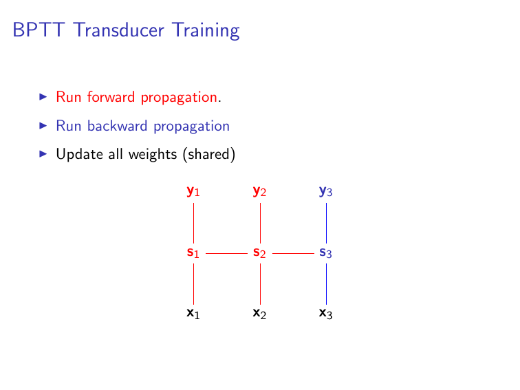
In this case, you generally want the final layer of your network to be something like an nn.Sequencer(nn.LogSoftMax()), which will give a vector of predictions $\mathbf{y}_i$ for each time-step, rather than the un-Sequencered nn.SelectTable that we used in the acceptor case.
For training, the RNN library also makes available a SequencerCriterion, which you can feed the (table of) output predictions of your network to. For example, you can use a SequencerCriterion as follows:
crit = nn.SequencerCriterion(nn.ClassNLLCriterion())
Using a SeqencerCriterion's :backward() function will allow you to generate a gradOutput that has nonzero values at all timesteps, as you'd expect for a transducer RNN.
Extensions/Advanced Topics
Stacking RNNs
An additional benefit of the nn.Sequencer decorator is that it allows for easily stacking RNNs. When RNNs are stacked, the hidden state of the $i$'th time-step at the $l$'th layer is calculated using the hidden-state at the $i$'th time-step from $l-1$'th layer (i.e., the previous layer) as input, and the hidden-state at the $i-1$'th time-step from the $l$'th layer (i.e., the current layer) as the previous hidden state. Formally, we use the following recurrence
\begin{align*} \mathbf{s}_{i}^{(l)} = R(\mathbf{s}_{i}^{(l-1)}, \mathbf{s}_{i-1}^{(l)}; \mathbf{\theta}), \end{align*}where we must define initial vectors $\mathbf{s}_{0}^{(l)}$ for all layers $l$, and where $\mathbf{s}_{i}^{(0)} = \mathbf{x}_i$. That is, we consider the first layer to just be the input.
Let's see this in action.
stackedSongLSTM = nn.Sequential():add(LT):add(nn.SplitTable(1, 3))
stackedSongLSTM:add(nn.Sequencer(nn.LSTM(embed_dim, embed_dim))) -- add first layer
stackedSongLSTM:add(nn.Sequencer(nn.LSTM(embed_dim, embed_dim))) -- add second layer
print(stackedSongLSTM:forward(songDataT))
{
  1 : DoubleTensor - size: 3x6
  2 : DoubleTensor - size: 3x6
  3 : DoubleTensor - size: 3x6
  4 : DoubleTensor - size: 3x6
  5 : DoubleTensor - size: 3x6
}
-- let's make sure the recurrences happened as we expect
-- as a sanity check, let's print out the embeddings we sent into the lstm
print(LT:forward(songDataT))
(1,.,.) =
  0.0207 -0.3298  0.4241 -0.0329 -0.4828  0.4233
 -0.8450 -0.9751 -0.0839 -0.0505 -0.4187 -0.3214
 -1.2384 -0.9624  0.5355  0.6253 -2.0640 -0.1330

(2,.,.) =
 -2.2302 -0.4697  1.2231 -0.5684  0.7322  0.3171
  1.2962 -1.2254  1.1809 -0.9699  0.7855 -1.3677
 -1.1605  1.6948 -1.1619  0.6787  1.5540 -0.1504

(3,.,.) =
  0.8532 -1.7503  1.4326  0.4153  0.5067 -0.9556
 -1.3679 -0.0924  0.4910  0.3140  0.1526  1.8399
 -1.0243  1.5654 -1.4497 -1.8515  0.2037  0.8241

(4,.,.) =
  0.3506 -0.2661  0.2084  0.8789 -0.1744  0.3886
 -1.2801 -0.2434  0.8133  0.0314 -2.1498 -0.2125
  0.8638  1.2091 -1.0203 -0.6000  0.7709  0.6464

(5,.,.) =
  0.6819  0.0802 -2.0248  1.0273 -0.5064  1.1698
  0.0693  0.4376  0.2075 -0.1351 -0.0796  0.4734
  1.3427  0.7881  1.1979  0.6048 -0.2020  1.6119
[torch.DoubleTensor of size 5x3x6]
-- now let's look at the first layer LSTM's input at the third time-step; should match 3rd thing in the above!
firstLayerLSTM = stackedSongLSTM:get(3):get(1) -- Sequencer was 3rd thing added, and its first child is the LSTM
print(firstLayerLSTM.inputs[3])
 0.8532 -1.7503  1.4326  0.4153  0.5067 -0.9556
-1.3679 -0.0924  0.4910  0.3140  0.1526  1.8399
-1.0243  1.5654 -1.4497 -1.8515  0.2037  0.8241
[torch.DoubleTensor of size 3x6]
-- now let's look at the first layer LSTM's output at the 3rd time-step
print(firstLayerLSTM.outputs[3])
 0.3659 -0.0541 -0.0975  0.0482  0.2729  0.1363
 0.0825  0.0026  0.1654 -0.0329  0.0662  0.1808
 0.0515 -0.0234 -0.0917  0.1393 -0.0022 -0.2167
[torch.DoubleTensor of size 3x6]
-- let's now examine the second layer LSTM and its input
secondLayerLSTM = stackedSongLSTM:get(4):get(1)
print(secondLayerLSTM.inputs[3]) -- should match the OUTPUT of firstLayerLSTM at 3rd timestep
 0.3659 -0.0541 -0.0975  0.0482  0.2729  0.1363
 0.0825  0.0026  0.1654 -0.0329  0.0662  0.1808
 0.0515 -0.0234 -0.0917  0.1393 -0.0022 -0.2167
[torch.DoubleTensor of size 3x6]
When stacking LSTMs, it's common to put Dropout in between layers, which would look like this:
stackedSongLSTMDO = nn.Sequential():add(LT):add(nn.SplitTable(1, 3))
stackedSongLSTMDO:add(nn.Sequencer(nn.LSTM(embed_dim, embed_dim))) -- add first layer
stackedSongLSTMDO:add(nn.Sequencer(nn.Dropout(0.5)))
stackedSongLSTMDO:add(nn.Sequencer(nn.LSTM(embed_dim, embed_dim))) -- add second layer
print(stackedSongLSTMDO:forward(songDataT))
{
  1 : DoubleTensor - size: 3x6
  2 : DoubleTensor - size: 3x6
  3 : DoubleTensor - size: 3x6
  4 : DoubleTensor - size: 3x6
  5 : DoubleTensor - size: 3x6
}
Remembering and Forgetting
When training an RNN, the training-loop usually looks like the following (in pseudocode):
while stillInEpoch do
    batch = next batch of sequence-length x batch-size inputs
    lstm:forward(batch)
    gradOuts = gradOutput for each time-step (for each thing in the batch)
    lstm:backward(batch, gradOuts)
end
The sequence-length we choose to predict (and backprop through), however, is often shorter than the true length of the naturally occurring sequence it participates in. For example, we might imagine trying to train on 5-word windows of entire songs. In this case, we might arrange our data as follows:
| Sequence1 | Sequence2 |
|---|---|
| Hey | Set |
| I | fire |
| just | to |
| met | the |
| you | rain |
| And | Watched |
| this | it |
| is | pour |
| crazy | as |
| but | I |
| ... | ... |
where every 5th word is bolded. (Note that this data format is the transpose of the way your homework data is given).
Suppose now that we've just predicted and backprop'd through the first batch (of size 2), which consists of "Hey I just met you" and "Set fire to the rain." The second batch will then consist of "And this is crazy but" and "Watched it pour as I," respectively. When we start to predict on the first words of the second batch (namely, "And" and "Watched"), however, do we want to compute $\mathbf{s}_{And}$ and $\mathbf{s}_{Watched}$ using the final hidden states from the previous batch (namely, $\mathbf{s}_{you}$ and $\mathbf{s}_{rain}$) as our $\mathbf{s}_{i-1}$, or do we want to treat $\mathbf{s}_{And}$ and $\mathbf{s}_{Watched}$ as though they begin their own sequences, and simply use $\mathbf{s}_0$ as their respective $\mathbf{s}_{i-1}$?
The answer may depend on your application, but often (such as in language modeling), we choose a relatively short sequence-length for convenience, even though we are interested in modeling the much longer sequence as a whole. In this case, it might make sense to "remember" the final state from the previous batch. You can control this behaviour with a Sequencer's :remember() and :forget() functions, as follows:
-- let's make another LSTM
rememberLSTM = nn.Sequential():add(LT):add(nn.SplitTable(1, 3))
seqLSTM = nn.Sequencer(nn.LSTM(embed_dim, embed_dim))
-- possible arguments for :remember() are 'eval', 'train', 'both', or 'neither', which tells it whether to remember
-- only during evaluation (but not training), only during training, both or neither
seqLSTM:remember('both')  -- :remember() typically needs to only be called once
rememberLSTM:add(seqLSTM)

--since we're remembering, we expect inputting the same sequence twice in a row to give us different outputs
-- (since the first time the pre-first state is the zero vector, and the second it's the end of the sequence)
print(rememberLSTM:forward(songDataT)[5]) -- printing out just the final time-step

-- let's do it again with the same sequence!
print(rememberLSTM:forward(songDataT)[5]) -- printing out just the final time-step
 0.0227  0.1013  0.3024 -0.2104  0.2013 -0.2100
 0.0657  0.0732  0.0574  0.0041 -0.0855 -0.1164
 0.1384  0.1797 -0.0188 -0.3070  0.1675 -0.1781
[torch.DoubleTensor of size 3x6]
 0.0214  0.1109  0.3236 -0.2431  0.2091 -0.2093
 0.0673  0.0749  0.0669  0.0089 -0.0869 -0.1167
 0.1355  0.1898 -0.0217 -0.3160  0.1785 -0.1781
[torch.DoubleTensor of size 3x6]
-- we can forget our history, though, by calling :forget()
seqLSTM:forget()
print(rememberLSTM:forward(songDataT)[5]) -- printing out just the final time-step
 0.0227  0.1013  0.3024 -0.2104  0.2013 -0.2100
 0.0657  0.0732  0.0574  0.0041 -0.0855 -0.1164
 0.1384  0.1797 -0.0188 -0.3070  0.1675 -0.1781
[torch.DoubleTensor of size 3x6]
-- if we use :remember('neither') or :remember('eval'), :forget() is called internally before each :forward()
seqLSTM:remember('neither')
print(rememberLSTM:forward(songDataT)[5]) -- printing out just the final time-step
-- now it doesn't change if we call forward twice
print(rememberLSTM:forward(songDataT)[5]) -- printing out just the final time-step
 0.0227  0.1013  0.3024 -0.2104  0.2013 -0.2100
 0.0657  0.0732  0.0574  0.0041 -0.0855 -0.1164
 0.1384  0.1797 -0.0188 -0.3070  0.1675 -0.1781
[torch.DoubleTensor of size 3x6]
 0.0227  0.1013  0.3024 -0.2104  0.2013 -0.2100
 0.0657  0.0732  0.0574  0.0041 -0.0855 -0.1164
 0.1384  0.1797 -0.0188 -0.3070  0.1675 -0.1781
[torch.DoubleTensor of size 3x6]
N.B.
- Even though it's useful to know about and understand :remember() and :forget(), you will mostly be using :remember() (at least in homework)