Quantum Circuit Plotting with SymPy¶

Rick Muller, rpmuller@gmail.com

Explore what can and cannot be done using existing sympy circuit plotting. The initial aim will be to support everything that is on the qasm2circ website. When you see a heading listing an example number, it will refer to the example circuit on that page.

Note: The examples on this page will require at least the development (i.e. github) branch of sympy, and may require work in my current branch (which changes from week to week). If you'd like to play with newer features, and the examples on this page aren't working for you, email me (rpmuller@gmail.com) and I can send you instructions for how to get these to work.

In [1]:

from sympy import *
from sympy.physics.quantum.circuitplot import CircuitPlot,labeller,Mz,CreateOneQubitGate
from sympy.physics.quantum.gate import *
from sympy.physics.quantum.qasm import Qasm

Rough priorities of tasks¶

Stack multiple gates vertically
Block multiqubit gate
Latex matrices as gates
Do circuits resize correctly?

Qasm tests status¶

Works
Works
Works
Works
Can't plot matrices as operators
Works
Works
Works
Works
Multi-qubit blocks + classical lines
Multi-qubit blocks
Multi-qubit blocks
Multi-qubit blocks (kinda works if you convert defbox->def by hand)
Multi-qubit blocks
D-shaped measurement
D-shaped measurement + slash gate + vertical line gates
D-shaped measurement

X gate test¶

In [2]:

CircuitPlot(CNOT(1,0),2)

Out[2]:

<sympy.physics.quantum.circuitplot.CircuitPlot at 0x103844f90>

In [3]:

CircuitPlot(X(0),1)

Out[3]:

<sympy.physics.quantum.circuitplot.CircuitPlot at 0x104dec090>

Sympy now prints a normal X gate when it's a one-qubit gate, but the circ+ when it's a CNOT!

Z gate test¶

In [4]:

CircuitPlot(CPHASE(1,0),2)

Out[4]:

<sympy.physics.quantum.circuitplot.CircuitPlot at 0x104e03d10>

In [5]:

CircuitPlot(Z(0),1)

Out[5]:

<sympy.physics.quantum.circuitplot.CircuitPlot at 0x104ecba90>

Making arbitrary gates:¶

It's pretty easy to overload single-qubit operators, and you can even specify fairly complicated LaTeX:

In [6]:

VGate = CreateOneQubitGate('V')
SqrtX = CreateOneQubitGate('sqrt-X','\sqrt{X}')

In [7]:

CircuitPlot(SqrtX(0)*VGate(0),1)

Out[7]:

<sympy.physics.quantum.circuitplot.CircuitPlot at 0x104ee3b10>

You can even make these controlled:

In [8]:

CircuitPlot(CGate(1,SqrtX(0)),2)

Out[8]:

<sympy.physics.quantum.circuitplot.CircuitPlot at 0x104e7d690>

Unfortunately, there isn't a general way to make a block multi-qubit gate. You need to overload the plot_gate function, which I haven't. And, I guess you also have to make sure that all of the qubits are contiguous.

Todo Create multi-qubit gate.

In [9]:

class SqrtSWAP(TwoQubitGate):
    gate_name = 'sqrt-SWAP'
    gate_name_latex = u'\sqrt{SWAP}'

In [10]:

# This doesn't work:
# CircuitPlot(SqrtSWAP(0,1),2)

Example 1: EPR Creation¶

Goal:

In [11]:

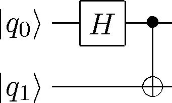
CircuitPlot(CNOT(1,0)*H(1),2,labels=labeller(2))

Out[11]:

<sympy.physics.quantum.circuitplot.CircuitPlot at 0x104ef0e50>

A couple of notes:

The top wire in a figure is the nth qubit in the circuit, not the 0-th or 1st.
The gates in a circuit are ordered left to right. In other words, the first gate to be applied is the left-most gate in the circuit.

Both of these make perfect sense from a physics point of view, but they may not be what you expect.

qasm version:¶

In [12]:

q = Qasm('qubit q0','qubit q1','h q0','cnot q0,q1')
q.plot()

Works, but note that I haven't implemented the subscripts in qasm parser yet. It's not hard to rewrite the labelling so that it sticks an underscore between the alphabetical characters and the numbers, but I don't want to limit the way the code works based on assumptions of use cases that I haven't fully thought through. In the meantime, if you stick underscores in the label names, these will work:

In [13]:

q = Qasm('qubit q_0','qubit q_1','h q_0','cnot q_0,q_1')
q.plot()

You can also call the commands directly:

In [14]:

q = Qasm()
q.qubit('q_0')
q.qubit('q_1')
q.h('q_0')
q.cnot('q_0','q_1')
q.plot()

Example 2: Teleportation Gate¶

Goal:

In [15]:

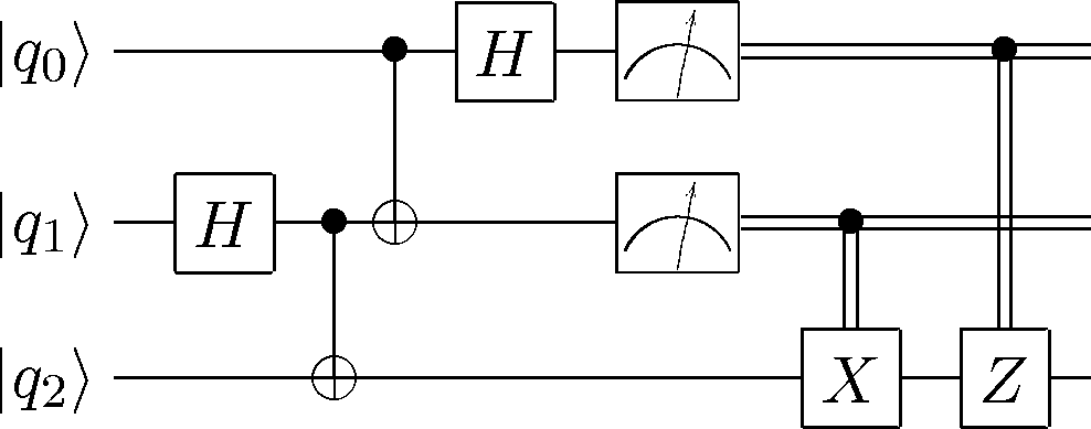
circuit = CGate(2,Z(0))*CGate(1,X(0))*Mz(2)*Mz(1)*H(2)*CNOT(2,1)*CNOT(1,0)*H(1)
cp = CircuitPlot(circuit,3,labels=labeller(3))

In [16]:

# qasm version
q = Qasm('qubit q_0','qubit q_1','qubit q_2','h  q_1',
         'cnot q_1,q_2','cnot q_0,q_1','h q_0',
         'measure q_1','measure q_0',
         'c-x q_1,q_2','c-z q_0,q_2')
q.plot()

Example 3: Swap Gate¶

Goal:

In [17]:

CircuitPlot(CNOT(1,0)*CNOT(0,1)*CNOT(1,0),2,labels=labeller(2))

Out[17]:

<sympy.physics.quantum.circuitplot.CircuitPlot at 0x104fae810>

qasm version:¶

In [18]:

q = Qasm('qubit q_0','qubit q_1','cnot q_0,q_1','cnot q_1,q_0','cnot q_0,q_1')
q.plot()

Example 4: QFT on 3 Qubits¶

Goal:

In [19]:

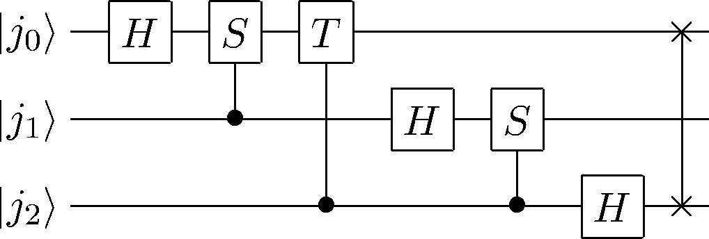
CircuitPlot(SWAP(0,2)*H(0)* CGate((0,),S(1)) *H(1)*CGate((0,),T(2))*CGate((1,),S(2))*H(2),3,labels=labeller(3,'j'))

Out[19]:

<sympy.physics.quantum.circuitplot.CircuitPlot at 0x104f7de50>

In [20]:

# qasm version:
q = Qasm("def	c-S,1,'S'",
        "def	c-T,1,'T'",
        "qubit	j0",
        "qubit	j1",
        "qubit	j2",
        "h	j0",
        "c-S	j1,j0",
        "c-T	j2,j0",
        "nop	j1",
        "h	j1",
        "c-S	j2,j1",
        "h	j2",
        "swap	j0,j2")
q.plot()

Example 5¶

Goal:

In [21]:

# Note: you currently have to escape (double backslash) the \b and \t, 
# I guess b/c they're whitespace shortcuts
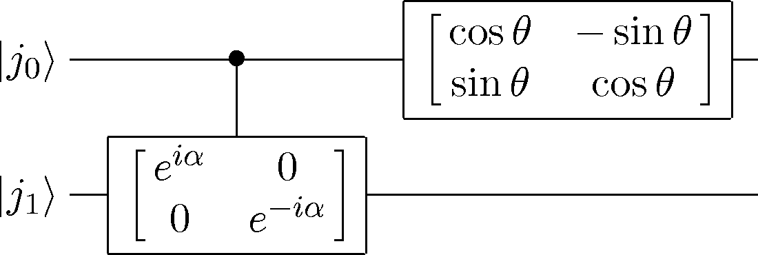
class Rot1(OneQubitGate):
    gate_name = 'Rot'
    gate_name_latex = r'\begin{array}{ll}\cos\theta&-\sin\theta\end{array}'

In [22]:

# This doesn't work:
#CircuitPlot(Rot1(0),1)

Example 6¶

Goal:

In [23]:

U = CreateOneQubitGate('U')
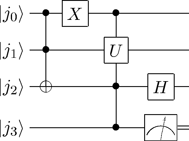
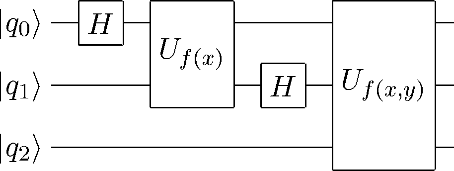
CircuitPlot(Mz(0)*H(1)*CGate((0,1,3),U(2))*X(3)*CGateS((2,3),X(1)),4,labels=labeller(4,'j'))

Out[23]:

<sympy.physics.quantum.circuitplot.CircuitPlot at 0x104e68c90>

In [24]:

# Qasm version:
q = Qasm("def	c-U,3,'U'",
    "qubit	j0",
    "qubit	j1",
	"qubit	j2",
    "qubit	j3",
    "toffoli	j0,j1,j2",
    "X	j0",
    "c-U	j2,j3,j0,j1",
    "H	j2",
    "measure	j3")
q.plot()

Example 7¶

Goal:

In [25]:

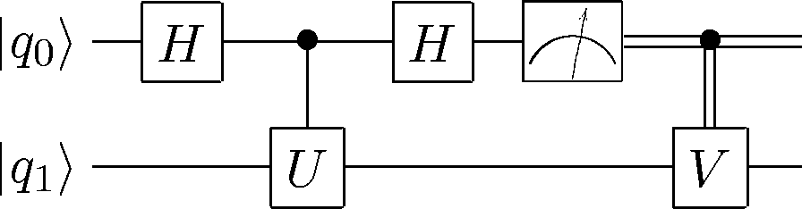
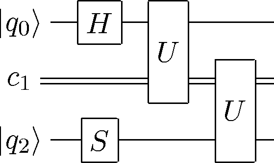
V = CreateOneQubitGate('V')

CircuitPlot(CGate(1,V(0))*Mz(1)*H(1)*CGate(1,U(0))*H(1),2,labels=labeller(2))

Out[25]:

<sympy.physics.quantum.circuitplot.CircuitPlot at 0x10515b450>

In [26]:

# Qasm
q = Qasm("def	c-U,1,'U'","def	c-V,1,'V'",
         "qubit	q0","qubit	q1",
         "H	q0","c-U	q0,q1","H	q0",
         "measure	q0","c-V	q0,q1")
q.plot()

Example 8¶

Goal:

In [27]:

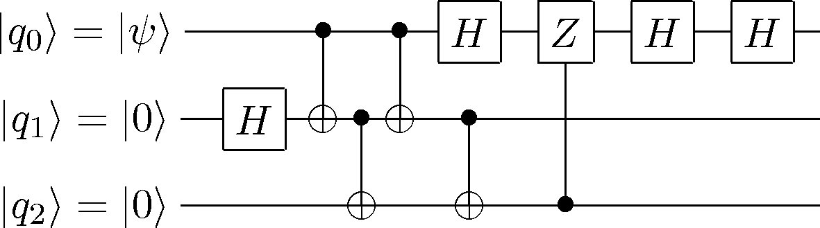
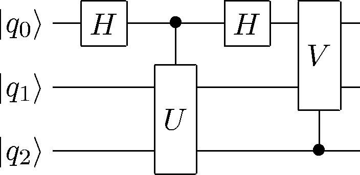
CircuitPlot(H(2)*H(2)*CGate(0,Z(2))*H(2)*CNOT(1,0)*CNOT(2,1)*CNOT(1,0)*CNOT(2,1)*H(1),3,labels=labeller(3))

Out[27]:

<sympy.physics.quantum.circuitplot.CircuitPlot at 0x105104c50>

In [28]:

#Qasm:
q = Qasm("def	c-Z,1,'Z'",
         "qubit	q0,\psi","qubit	q1,0","qubit	q2,0",
         "H	q1","cnot	q0,q1","cnot	q1,q2","cnot	q0,q1","cnot	q1,q2",
         "H	q0","c-Z	q2,q0","H	q0","H	q0")
q.plot()

Example 9¶

Goal:

In [29]:

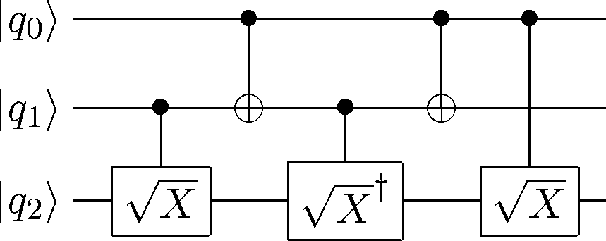
SqrtX = CreateOneQubitGate('sqrt-X','\sqrt{X}')
SqrtXdag = CreateOneQubitGate('sqrt-X-dag','\sqrt{X}^\dagger')

CircuitPlot(CGate(2,SqrtX(0))*CNOT(2,1)*CGate(1,SqrtXdag(0))*CNOT(2,1)*CGate(1,SqrtX(0)),3,labels=labeller(3))

Out[29]:

<sympy.physics.quantum.circuitplot.CircuitPlot at 0x104f62a10>

In [30]:

q = Qasm("def	c-X,1,'\sqrt{X}'","def	c-Xd,1,'{\sqrt{X}}^\dagger'",
         "qubit	q0","qubit	q1","qubit	q2",
         "c-X	q1,q2","cnot	q0,q1","c-Xd	q1,q2",
         "cnot	q0,q1","c-X	q0,q2")
q.plot()

Example 10¶

Goal:

Example 11¶

Goal:

Example 12¶

Goal:

Example 13¶

Goal:

In [40]:

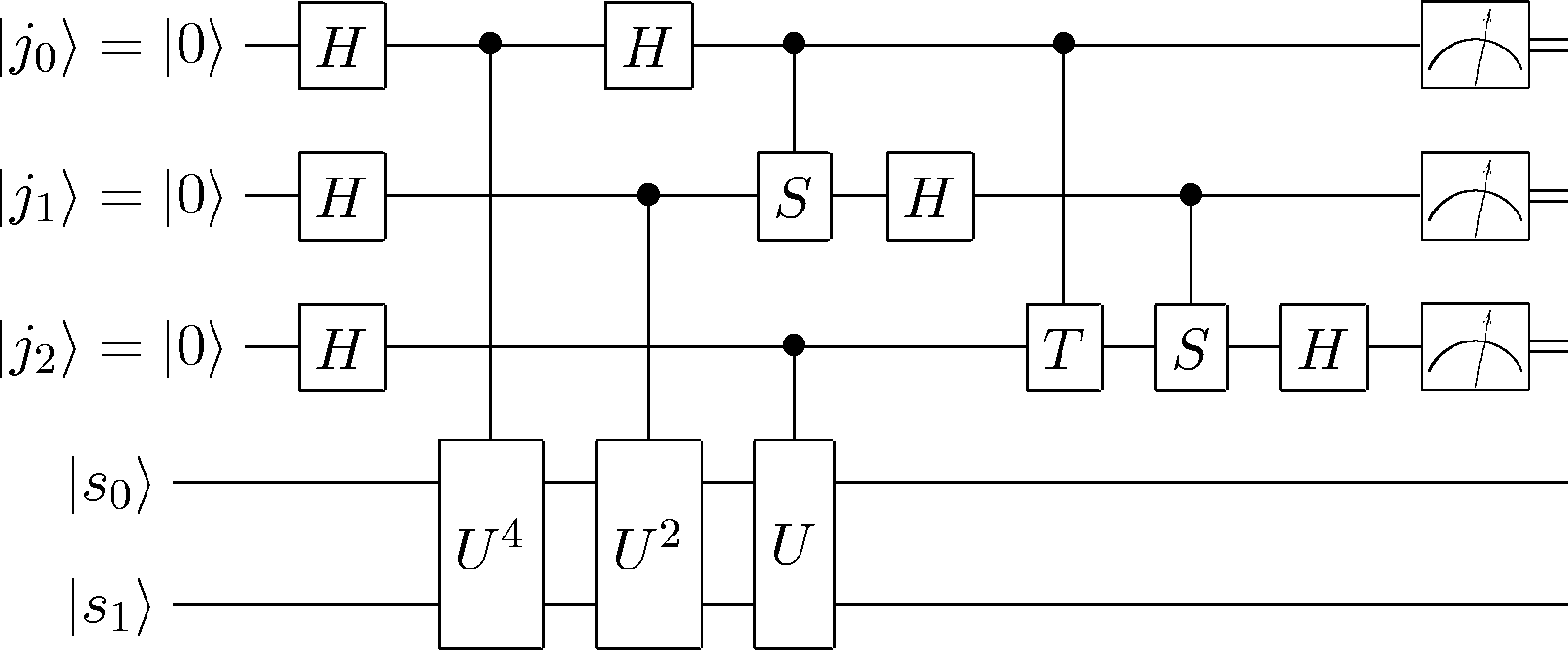
# Only works if you convert the defboxes to defs and remove qubit s2:
qasm_lines = """\
	def	CU,1,'U'
	def	CU2,1,'U^2'
	def	CU4,1,'U^4'
	def	c-S,1,'S'
	def	c-T,1,'T'

	qubit	j0,0	# QFT qubits
	qubit	j1,0
	qubit	j2,0
	qubit	s0	# U qubits

	h	j0	# equal superposition
	h	j1
	h	j2

	CU4	j0,s0	# controlled-U
	CU2	j1,s0
	CU	j2,s0

	h	j0	# QFT
	c-S	j0,j1
	h	j1
	nop	j0
	c-T	j0,j2
	c-S	j1,j2
	h	j2
	nop	j0
	nop	j0
	nop	j1
	
	measure	j0	# final measurement
	measure	j1	
	measure	j2"""

q = Qasm(*qasm_lines.splitlines())
q.plot()

Example 14¶

Goal:

Example 15¶

Goal:

In [31]:

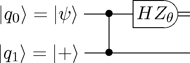
CircuitPlot(Mz(1)*CPHASE(0,1),2,labels=['+','\psi'])

Out[31]:

<sympy.physics.quantum.circuitplot.CircuitPlot at 0x10544ba90>

Example 16¶

Goal:

In [32]:

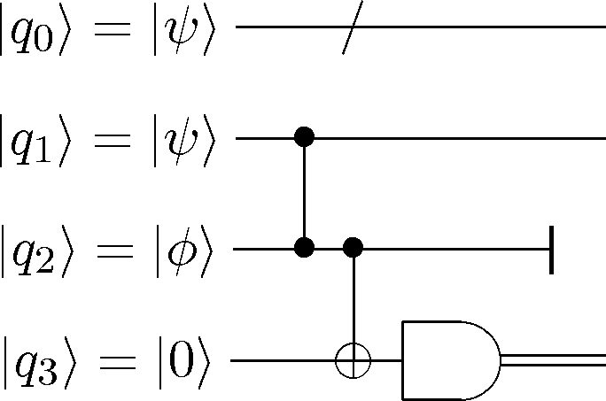
CircuitPlot(Mz(0)*CNOT(1,0)*CPHASE(1,2),4,labels=['0','\phi','\psi','\psi'])

Out[32]:

<sympy.physics.quantum.circuitplot.CircuitPlot at 0x105607bd0>

Example 17¶

Goal:

In [33]:

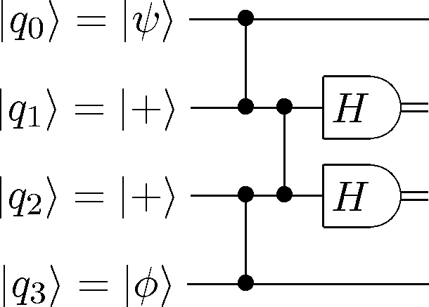
CircuitPlot(Mz(2)*Mz(1)*CPHASE(1,2)*CPHASE(1,0)*CPHASE(3,2),4,labels=['\phi','+','+','\psi'])

Out[33]:

<sympy.physics.quantum.circuitplot.CircuitPlot at 0x1050f53d0>

Surface code¶

These are the X and Z checks from a surface code:

In [34]:

CircuitPlot(Mz(4)*H(4)*CNOT(4,0)*CNOT(4,1)*CNOT(4,2)*CNOT(4,3)*H(4),5,labels=['d_4','d_3','d_2','d_1','a_0'])

Out[34]:

<sympy.physics.quantum.circuitplot.CircuitPlot at 0x105701350>

In [35]:

CircuitPlot(Mz(4)*CNOT(0,4)*CNOT(1,4)*CNOT(2,4)*CNOT(3,4),5,labels=['d_4','d_3','d_2','d_1','a_0'])

Out[35]:

<sympy.physics.quantum.circuitplot.CircuitPlot at 0x104fc2b10>

Steane code¶

Make $|\bar{0}\rangle$ , Fig 12 from Aliferis, Gottesman, and Preskill.

In [36]:

CircuitPlot(CNOT(6,0)*CNOT(5,4)*CNOT(3,2)*CNOT(5,1)*CNOT(3,0)*CNOT(6,2)*CNOT(6,4)*CNOT(3,0),
    7,labels=["0","0","0","+","0","+","+"])

Out[36]:

<sympy.physics.quantum.circuitplot.CircuitPlot at 0x105862d50>

Let's use the power of python to make this a little easier:

In [37]:

import operator
def prod(c): return reduce(operator.mul, c, 1)

steane_pairs = [(6,0),(5,4),(3,2),(5,1),(3,0),(6,2),(6,4),(3,0)]
circuit2 = prod([CNOT(i,j) for i,j in steane_pairs])
labels=["0","0","0","+","0","+","+"]
CircuitPlot(circuit2,7,labels=labels)

Out[37]:

<sympy.physics.quantum.circuitplot.CircuitPlot at 0x1059d0b50>

We can now extend this to a full Steane check:

In [38]:

circuit1 = prod([CNOT(i+7,j+7) for i,j in steane_pairs])
decoder = prod([CNOT(i+7,j+7) for i,j in reversed(steane_pairs)])
transverse = prod([CPHASE(i+7,i) for i in range(7)])
CircuitPlot(decoder*transverse*circuit2*circuit1,14,labels=labels+labels)

Out[38]:

<sympy.physics.quantum.circuitplot.CircuitPlot at 0x1059c6b90>

That's only 7 real lines of code to plot the encoding.

In [38]: