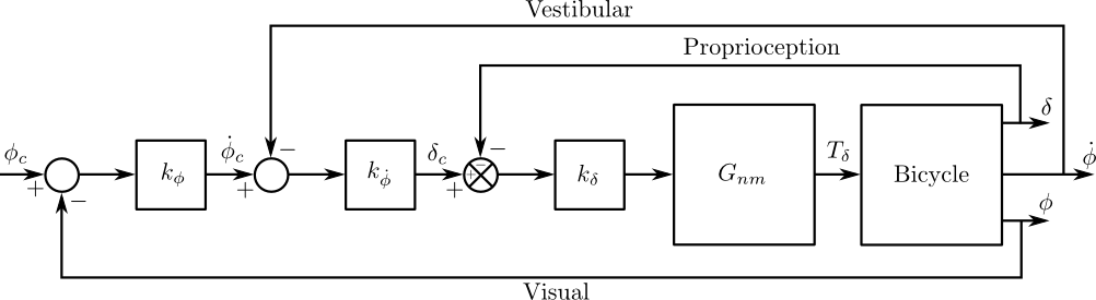
This document describes an attempt to solve for the gains of the first two loops of this block diagram to ensure that at a pair of the poles end up in a desired location.
where
$$G_{nm}(s) = \frac{\omega_{nm}^2}{s^2 + 2\zeta_{nm}\omega_{nm}s + \omega_{nm}^2}$$and the bicycle block is the linearized Whipple model as presented in Meijaard 2007.
Setup
import os
import dill
from IPython.display import display, Math
from sympy import MatrixSymbol, Eq, simplify, Poly, det, latex, S, solve, cse
from dtk import bicycle
import bicycleparameters as bp
The roll_rate_loop.py file builds the bicycle state space, the neuromuscular state space, and finally the state equations for the closed loop system when the steering angle and roll rate feedback loops are closed.
%run roll_rate_loop.py
State Space Definitions
The bicycle state equations take this general form:
[Eq(MatrixSymbol('{}_b'.format(v), *b[v].shape), b[v]) for v in ['A', 'x', 'B', 'u']]
The second order neuromuscular model can be put in this state space form:
[Eq(MatrixSymbol('{}_nm'.format(v), *n[v].shape), n[v]) for v in ['A', 'x', 'B', 'u']]
The closed loop state equations for the first two loops that are closed around the combine neuromuscular and bicycle model then become:
[Eq(MatrixSymbol('{}_cl'.format(v), *c[v].shape), c[v]) for v in ['A', 'x', 'B', 'u']]
Characteristic Equation
The characteristic equation can be formed for this closed loop system and converted to a polynomial.
s = Symbol('s')
char_eq = det(c['A'] - s * eye(c['A'].shape[0])).as_poly(s)
char_eq
Additionally, the coefficients to the 6th order polynomial can be extracted and simplified:
for i, coeff in enumerate(char_eq.coeffs()):
    display(Math(r'$s^{}: {}$'.format(len(char_eq.coeffs()) - i - 1, latex(simplify(coeff)))))
The symbolic form of the characteristic equation cannot be easily factored.
char_eq.factor()
Solve for the gains
There are two control gains, $k_\delta$ and $k_{\dot{\phi}}$, that are the unknowns. We'd like to find the value of the two gains such that the weave poles when there is no feedback, i.e. $k_\delta=0$ and $k_{\dot{\phi}}=0$, shift to a pair of poles when there is feedback that are located at a damping ratio of 0.15 and a natural frequency of 10 rad/s. This pair of poles gives a desired second order system:
desired_second_order = Poly((s**2 + 2 * S(15)/100 * 10 * s + 10**2), s)
desired_second_order
This pair of poles must be accompanied by four more poles to equate to the sixth order system above. The desired sixth order system with arbitrary coefficients is then:
c0, c1, c2, c3 = symbols('c0, c1, c2, c3')
desired_six_order = Poly(s**4 + c3 * s**3 + c2 * s**2 + c1 * s + c0, s) * desired_second_order
desired_six_order
The coefficients of the desired polynomial and the one formed from the closed loop system can then be substracted from each other to solve for the unknowns: $c_0, c_1, c_2, c_3, k_\delta, k_{\dot{\phi}}$. This gives 6 equations for the six unknowns.
zero = Matrix((char_eq - desired_six_order).coeffs())
zero
The following loads in the numerical parameters for the benchmark bicycle traveling at 5 m/s, for futher use.
A_benchmark, B_benchmark = bicycle.benchmark_state_space(*bicycle.benchmark_matrices(), 5.0, 9.81)
A_benchmark, B_benchmark
(array([[  0.        ,   0.        ,   1.        ,   0.        ],
        [  0.        ,   0.        ,   0.        ,   1.        ],
        [  9.48977445, -22.85146663,  -0.52761225,  -1.65257699],
        [ 11.71947687, -18.38412373,  18.38402617, -15.42432764]]),
 array([[ 0.        ,  0.        ],
        [ 0.        ,  0.        ],
        [ 0.01593498, -0.12409203],
        [-0.12409203,  4.32384018]]))
Create a dictionary that can be used to substitute the numerical values for the benchmark bicycle.
par = {k: v for k, v in zip(b['A'], A_benchmark.flatten()) if isinstance(k, Symbol)}
par[omega] = 30
par[zeta] = 0.707
par[b['B'][2, 1]] = B_benchmark[2, 1]
par[b['B'][3, 1]] = B_benchmark[3, 1]
par
The following shows the form of the six equations that must be solved to find the gains and the other coefficients. The equations are linear in the $c$ coefficients and nonlinear in the gains. Notice that the gains are only in the last four equations.
zero.subs(par)
Now we can attempt to solve for the gains analytically. This set of equations are polynomials in the unknowns and may have an analytica solution. First we solve the first two linear equations for $c_2$ and $c_3$ and substitute them into the last four equations.
c2_c3_sol = solve(zero[:2], c2, c3)
c2_c3_sol
lastfour = simplify(zero[2:, :].subs(c2_c3_sol))
lastfour
The following caches the result of the solve command to disk because it takes so long (about 4 hours on my machine) to compute.
CPU times: user 3h 56min 9s, sys: 832 ms, total: 3h 56min 10s
Wall time: 3h 56min 12s
%%time

fname = "sol.p"

if os.path.isfile(fname):
    with open(fname, 'rb') as f:
        sol = dill.load(f)
else:
    sol = solve(lastfour, c0, c1, k_delta, k_phi_dot)
    with open(fname, "wb") as f:
        dill.dump(sol, f)
CPU times: user 424 ms, sys: 4 ms, total: 428 ms
Wall time: 430 ms
The solution is returned as a list of lists, so stick it in a dictionary for future use.
sol = {k: v for k, v in zip((c0, c1, k_delta, k_phi_dot), sol[0])}
Generate a Python function
Next I generate an efficient Python function that evaluates the found expressions for $k_\delta$ and $k_\dot{\phi}$.
py_func_template = '''\
def compute_inner_gains(A, B, omega_nm, zeta_nm):
    """Returns the steer and roll rate gains given the state and input
    matrices of the bicycle and the neuromuscular block's natural
    frequency and damping ratio.

    Parameters
    ==========
    A : array_like, shape(4, 4)
        The state matrix for a linear Whipple bicycle model, where
        the states are [roll angle, steer angle, roll angular rate,
        steer angular rate].
    B : array_like, shape(4, 2)
        The input matrix for a linear Whipple bicycle model, where
        the inputs are [roll torque, steer torque].
    omega_nm : float
        The natural frequency of the neuromuscular model.
    zeta_nm : float
        The damping ratio of the neuromuscular model.

    Returns
    =======
    k_delta : float
        The steer angle feedback gain.
    k_phi_dot : float
        The roll rate feedback gain.

    """
    {matrix_expansion}

    {sub_exprs}

{main_exprs}

    return k_delta, k_phi_dot\
'''
sub_exprs, main_exprs = cse([sol[k_delta], sol[k_phi_dot]])
zero_syms = zero.free_symbols
matrix_expansion = []
for mat in ['A', 'B']:
    for i, row in enumerate(b[mat].tolist()):
        for j, col in enumerate(row):
            if col in zero_syms:
                matrix_expansion.append('{} = {}[{}, {}]'.format(col, mat, i, j))
sub_exprs_txt = ['{} = {}'.format(x, y) for x, y in sub_exprs]
main_exprs_txt = ' k_delta = {}\n\n k_phi_dot = {}'.format(*main_exprs)
The full function is shown below:
func_txt = py_func_template.format(matrix_expansion='\n    '.join(matrix_expansion),
                              sub_exprs='\n    '.join(sub_exprs_txt),
                              main_exprs=main_exprs_txt)
print(func_txt)
def compute_inner_gains(A, B, omega_nm, zeta_nm):
    """Returns the steer and roll rate gains given the state and input
    matrices of the bicycle and the neuromuscular block's natural
    frequency and damping ratio.

    Parameters
    ==========
    A : array_like, shape(4, 4)
        The state matrix for a linear Whipple bicycle model, where
        the states are [roll angle, steer angle, roll angular rate,
        steer angular rate].
    B : array_like, shape(4, 2)
        The input matrix for a linear Whipple bicycle model, where
        the inputs are [roll torque, steer torque].
    omega_nm : float
        The natural frequency of the neuromuscular model.
    zeta_nm : float
        The damping ratio of the neuromuscular model.

    Returns
    =======
    k_delta : float
        The steer angle feedback gain.
    k_phi_dot : float
        The roll rate feedback gain.

    """
    a_20 = A[2, 0]
    a_21 = A[2, 1]
    a_22 = A[2, 2]
    a_23 = A[2, 3]
    a_30 = A[3, 0]
    a_31 = A[3, 1]
    a_32 = A[3, 2]
    a_33 = A[3, 3]
    b_21 = B[2, 1]
    b_31 = B[3, 1]

    x0 = omega_nm**2
    x1 = 10000*b_31
    x2 = 91*b_31
    x3 = a_20*b_21
    x4 = 300*a_22*b_21
    x5 = 100*b_31
    x6 = a_31*b_21
    x7 = a_20*a_31*b_21
    x8 = a_21*b_31
    x9 = a_30*b_21
    x10 = b_31**2
    x11 = a_21*x10
    x12 = b_21**2
    x13 = a_30*x12
    x14 = 300*a_32
    x15 = 3*b_31
    x16 = a_20*a_33*b_21
    x17 = a_22*a_33*b_21
    x18 = a_23*a_30*b_21
    x19 = a_23*a_32*b_21
    x20 = a_23*x10
    x21 = 3*a_33
    x22 = 100*a_32
    x23 = 91000000*b_21
    x24 = 1000000*x3
    x25 = 738100*x8
    x26 = a_22*b_21
    x27 = 3000000*x26
    x28 = 5730000*b_31
    x29 = a_23*x28
    x30 = 1738100*x6
    x31 = a_33*b_21
    x32 = 2730000*x31
    x33 = a_20*a_21*b_31
    x34 = 9100*x33
    x35 = 30000*a_23
    x36 = a_20*b_31
    x37 = x35*x36
    x38 = 19100*x7
    x39 = 30000*x16
    x40 = 57300*a_21*b_31
    x41 = a_22*x40
    x42 = a_21*a_30*b_21
    x43 = 10000*x42
    x44 = a_21*a_31*b_31
    x45 = 9100*x44
    x46 = a_33*x40
    x47 = a_22*a_23*b_31
    x48 = 910000*x47
    x49 = 57300*a_22*b_21
    x50 = a_31*x49
    x51 = 90000*x17
    x52 = 30000*a_31*b_31
    x53 = a_23*x52
    x54 = 1000000*x19
    x55 = 910000*a_33*b_31
    x56 = a_23*x55
    x57 = 27300*a_33
    x58 = x57*x6
    x59 = b_21*omega_nm*zeta_nm
    x60 = 6000000*x59
    x61 = a_31**2
    x62 = 9100*b_21
    x63 = x61*x62
    x64 = a_33**2
    x65 = b_21*x64
    x66 = 910000*x65
    x67 = b_21*x0
    x68 = 1000000*x67
    x69 = 100*a_31
    x70 = x33*x69
    x71 = 300*a_33
    x72 = x33*x71
    x73 = 10000*a_23
    x74 = a_20*a_33*b_31
    x75 = x73*x74
    x76 = x7*x71
    x77 = 300*a_22
    x78 = x44*x77
    x79 = 9100*a_33
    x80 = a_21*a_22*b_31
    x81 = x79*x80
    x82 = a_21*a_23*a_30*b_31
    x83 = 300*x82
    x84 = a_21*a_23*a_32*b_31
    x85 = 900*x84
    x86 = x42*x69
    x87 = a_21*a_31*b_21
    x88 = x14*x87
    x89 = a_21*a_32*a_33*b_21
    x90 = 10000*x89
    x91 = 114600*omega_nm*zeta_nm
    x92 = x8*x91
    x93 = 10000*a_22*a_23*b_31
    x94 = a_31*x93
    x95 = a_22*a_33*b_31
    x96 = x35*x95
    x97 = 900*a_31
    x98 = x17*x97
    x99 = a_22*b_21*omega_nm*zeta_nm
    x100 = 2000000*x99
    x101 = 300*a_31
    x102 = x101*x18
    x103 = a_30*a_33*b_21
    x104 = x103*x73
    x105 = 9100*a_32
    x106 = x105*x6
    x107 = a_23*x106
    x108 = a_32*a_33*b_21
    x109 = x108*x35
    x110 = omega_nm*zeta_nm
    x111 = 1820000*b_31*x110
    x112 = a_23*x111
    x113 = x6*x91
    x114 = 180000*a_33*b_21*x110
    x115 = 100*x61
    x116 = x115*x3
    x117 = 10000*a_20*b_21
    x118 = x117*x64
    x119 = x0*x117
    x120 = 9100*x0
    x121 = x120*x8
    x122 = a_21**2
    x123 = a_30*x122
    x124 = x123*x5
    x125 = a_32*b_31*x122
    x126 = 300*x125
    x127 = x4*x61
    x128 = 30000*x26*x64
    x129 = b_31*x0
    x130 = x129*x35
    x131 = a_23**2
    x132 = a_30*x131
    x133 = x1*x132
    x134 = a_32*b_31*x131
    x135 = 30000*x134
    x136 = a_31*b_21*x0
    x137 = 19100*x136
    x138 = 30000*x0*x31
    x139 = 600*omega_nm*zeta_nm
    x140 = x139*x33
    x141 = 20000*a_23
    x142 = a_20*b_31*omega_nm*zeta_nm
    x143 = x141*x142
    x144 = 18200*omega_nm*zeta_nm
    x145 = x144*x80
    x146 = x139*x42
    x147 = x139*x44
    x148 = 20000*omega_nm*zeta_nm
    x149 = a_21*a_32*b_21
    x150 = x148*x149
    x151 = a_21*a_33*b_31*x144
    x152 = 60000*omega_nm*zeta_nm
    x153 = x152*x47
    x154 = a_22*a_31*b_21*omega_nm*zeta_nm
    x155 = 38200*x154
    x156 = x152*x17
    x157 = x148*x18
    x158 = b_31*omega_nm*zeta_nm
    x159 = 20000*a_31*x158
    x160 = a_23*x159
    x161 = 60000*a_33*x158
    x162 = a_23*x161
    x163 = 1800*omega_nm*zeta_nm
    x164 = a_31*a_33*b_21*x163
    x165 = 100*x0
    x166 = x165*x33
    x167 = 191*x0
    x168 = x167*x7
    x169 = 300*x0
    x170 = x16*x169
    x171 = x169*x80
    x172 = 91*x0
    x173 = x172*x42
    x174 = x165*x44
    x175 = x149*x169
    x176 = a_21*b_31*x0
    x177 = x176*x71
    x178 = x0*x93
    x179 = x169*x18
    x180 = 10000*x0
    x181 = x180*x19
    x182 = a_33*x0*x1
    x183 = a_23*x182
    x184 = x136*x71
    x185 = 600*b_21*omega_nm*zeta_nm
    x186 = x185*x61
    x187 = 60000*x59*x64
    x188 = 200*a_33*omega_nm*zeta_nm
    x189 = x188*x33
    x190 = a_20*a_31*b_31*omega_nm*zeta_nm
    x191 = 200*a_23*x190
    x192 = 200*a_22*omega_nm*zeta_nm
    x193 = x192*x44
    x194 = a_21*a_22*a_33*b_31
    x195 = x139*x194
    x196 = x139*x84
    x197 = x188*x42
    x198 = 200*a_32*omega_nm*zeta_nm
    x199 = x198*x87
    x200 = 20000*a_33*omega_nm*zeta_nm
    x201 = x200*x47
    x202 = a_22*a_31*a_33*b_21*x139
    x203 = 200*a_31*omega_nm*zeta_nm
    x204 = x18*x203
    x205 = a_23*a_31*a_32*b_21*x139
    x206 = x19*x200
    x207 = x115*x67
    x208 = x180*x65
    x209 = a_20*b_21*x0
    x210 = x209*x61
    x211 = x123*x129
    x212 = a_31*x0
    x213 = x212*x33
    x214 = 3*a_31
    x215 = a_20*a_23*b_31*x0*x214
    x216 = 100*a_23*x0
    x217 = x216*x74
    x218 = a_20*a_31*b_21*x0
    x219 = x21*x218
    x220 = x165*x194
    x221 = 3*x0
    x222 = x221*x82
    x223 = x212*x42
    x224 = a_21*a_30*b_21*x0*x21
    x225 = x165*x89
    x226 = 200*omega_nm*zeta_nm
    x227 = x125*x226
    x228 = a_22*a_23*b_31*x0
    x229 = x228*x69
    x230 = 200*x61*x99
    x231 = 20000*x64*x99
    x232 = x103*x216
    x233 = 100*a_23*a_32*x136
    x234 = x134*x148
    x235 = a_20*b_21*x165*x64
    x236 = 100*b_31*x0
    x237 = x132*x236
    x238 = a_22*b_31
    x239 = a_32*b_21
    x240 = a_20*a_30*b_21
    x241 = 573*a_31
    x242 = a_21*a_32*b_31
    x243 = a_22*a_30*b_21
    x244 = a_23*a_30
    x245 = a_20**2
    x246 = b_31*x245
    x247 = a_22**2
    x248 = b_31*x247
    x249 = 3*a_30
    x250 = a_20*a_21*a_32*b_31
    x251 = 9*a_20*a_22*b_31
    x252 = a_20*a_22*a_33*b_31
    x253 = a_20*a_23*a_30*b_31
    x254 = 573*a_20*b_31
    x255 = a_20*a_30*a_33*b_21
    x256 = a_21*a_22*a_30*b_31
    x257 = a_21*a_30*a_32*b_21
    x258 = a_22*a_23*a_30*b_31
    x259 = 91*a_22*a_30*b_21
    x260 = a_22*a_30*a_33*b_21
    x261 = 300*a_22*a_32*b_21
    x262 = a_22*b_31*omega_nm*zeta_nm
    x263 = a_23*a_30*a_32*b_21
    x264 = a_30*b_21*omega_nm*zeta_nm
    x265 = a_21*b_21
    x266 = a_30**2
    x267 = a_32**2
    x268 = a_22*b_31*x0
    x269 = a_23*x266
    x270 = a_23*x267
    x271 = a_30*b_21*x0
    x272 = a_20*a_22*b_31*omega_nm*zeta_nm
    x273 = 182*omega_nm*zeta_nm
    x274 = 600*a_32*omega_nm*zeta_nm
    x275 = 1146*omega_nm*zeta_nm
    x276 = a_30*omega_nm*zeta_nm
    x277 = 6*omega_nm*zeta_nm
    x278 = 18*omega_nm*zeta_nm
    x279 = 2*a_31*omega_nm*zeta_nm
    x280 = a_33*b_31*x245
    x281 = a_21*b_21*omega_nm*zeta_nm

    k_delta = (-x100 - x102 + x104 - x107 - x109 - x112 - x113 - x114 - x116 - x118 + x119 - x121 - x124 + x126 + x127 + x128 - x130 - x133 + x135 + x137 + x138 + x140 - x143 + x145 - x146 + x147 + x150 + x151 + x153 - x155 - x156 + x157 - x160 + x162 + x164 - x166 + x168 + x170 + x171 - x173 - x174 - x175 + x177 - x178 - x179 + x181 - x183 - x184 - x186 - x187 + x189 - x191 + x193 - x195 + x196 - x197 + x199 + x201 + x202 + x204 - x205 + x206 + x207 + x208 + x210 + x211 - x213 + x215 - x217 - x219 + x220 - x222 - x223 + x224 - x225 - x227 - x229 - x23 - x230 - x231 - x232 + x233 - x234 + x235 + x237 - x24 + x25 + x27 + x29 - x30 - x32 + x34 + x37 - x38 - x39 - x41 + x43 + x45 - x46 + x48 + x50 + x51 + x53 - x54 + x56 + x58 - x60 - x63 - x66 + x68 + x70 - x72 + x75 + x76 - x78 - x81 + x83 - x85 + x86 - x88 + x90 + x92 + x94 - x96 - x98)/(x0*(-a_20*x11 + 3*a_20*x20 - 100*a_22*x20 - a_31*x13 - a_33*x12*x22 + b_21*x1 + b_31*x4 + b_31*x7 - 100*x11 - x12*x14 + x13*x21 - 91*x13 - x15*x16 - x15*x18 + x17*x5 + x19*x5 + x2*x3 + x5*x6 + x8*x9))

    k_phi_dot = (2*a_20*a_21*b_31*x276 - 1719*a_20*a_22*b_31 - a_20*a_23*a_32*b_31*x221 + 200*a_21*b_31*x276 - a_22*a_30*a_31*b_21*x277 + a_22*a_33*b_21*x0*x22 - 182*a_23*a_32*x142 + a_23*a_32*x254 - a_31*x251 - a_31*x259 - a_31*x261 - 600*a_31*x262 + 182*a_31*x264 + 6*a_31*x272 - a_32*b_31*omega_nm*x141*zeta_nm + a_32*b_31*x35 + 200*a_32*x154 - a_32*x218 - a_32*x49 + 18200*a_32*x99 + a_33*b_31*x139*x247 + a_33*x2*x245 - a_33*x236*x247 + 6*b_21*omega_nm*x269*zeta_nm - 100*b_21*x0*x270 + 91*b_21*x269 + x0*x250 + x0*x251 + x0*x253 - x0*x254 + x0*x255 - x0*x256 + x0*x259 + x0*x261 - x0*x280 - x1*x244 + x101*x248 + x103*x172 - x103*x275 - 7381*x103 - x105*x17 + x105*x3 - x105*x47 + x106 + x108*x144 + x108*x169 - 57300*x108 - x111 - x120*x239 - 30000*x129 - x136*x22 - x14*x16 - 34762*x142 - x144*x248 - x159 + x16*x198 + x161 + x163*x95 + x165*x242 - x167*x74 - x169*x248 - x17*x274 - x176*x249 - x182 + x185*x270 - 382*x190 + x192*x242 - x203*x248 - x209*x22 + x212*x243 - x214*x240 + x214*x246 + x214*x271 + x22*x228 + x22*x7 + x221*x240 - x221*x246 + x221*x252 - x221*x260 + x221*x263 + x226*x258 + x236*x244 + x238*x57 + x238*x97 + 171900*x238 + x239*x91 + 738100*x239 + x240*x273 + x240*x279 - 573*x240 + x241*x36 - x241*x9 - x242*x77 - 10000*x242 - x243*x275 - 7381*x243 - x246*x273 - x246*x279 + 573*x246 + x248*x79 + 57300*x248 - x249*x33 - x250*x277 - 91*x250 - x252*x278 - 273*x252 - x253*x277 - 91*x253 - x255*x277 - 91*x255 + 100*x256 + x257*x277 - 9*x257 - 300*x258 - x260*x273 + 573*x260 - 54600*x262 - x263*x278 - 273*x263 + 14762*x264 + 3*x265*x266 + 300*x265*x267 - 2*x266*x281 - 200*x267*x281 - x268*x71 - 900*x268 - x269*x67 + x270*x62 + 573*x271 + 546*x272 + x274*x3 - x274*x47 + x274*x6 + x275*x74 + x277*x280 + x28 + 109443*x36 + x52 + x55 + 17381*x74 - 79443*x9)/(x100 + x102 - x104 + x107 + x109 + x112 + x113 + x114 + x116 + x118 - x119 + x121 + x124 - x126 - x127 - x128 + x130 + x133 - x135 - x137 - x138 - x140 + x143 - x145 + x146 - x147 - x150 - x151 - x153 + x155 + x156 - x157 + x160 - x162 - x164 + x166 - x168 - x170 - x171 + x173 + x174 + x175 - x177 + x178 + x179 - x181 + x183 + x184 + x186 + x187 - x189 + x191 - x193 + x195 - x196 + x197 - x199 - x201 - x202 - x204 + x205 - x206 - x207 - x208 - x210 - x211 + x213 - x215 + x217 + x219 - x220 + x222 + x223 - x224 + x225 + x227 + x229 + x23 + x230 + x231 + x232 - x233 + x234 - x235 - x237 + x24 - x25 - x27 - x29 + x30 + x32 - x34 - x37 + x38 + x39 + x41 - x43 - x45 + x46 - x48 - x50 - x51 - x53 + x54 - x56 - x58 + x60 + x63 + x66 - x68 - x70 + x72 - x75 - x76 + x78 + x81 - x83 + x85 - x86 + x88 - x90 - x92 - x94 + x96 + x98)

    return k_delta, k_phi_dot
Check the results
Here, I make use of the function to calculate the gains to see if it gives reasonable answers. First, see what kind of results are returned for the benchmark bicycle traveling at 5 m/s.
exec(func_txt)
k_delta_sol, k_phi_dot_sol = compute_inner_gains(A_benchmark, B_benchmark, 30, 0.707)
gain_sol = {k_delta: k_delta_sol, k_phi_dot: k_phi_dot_sol}
gain_sol
This is a good sign. The roll rate gain is found to be a small negative number and the steer rate gain is larger and positive. But the values that we find for our paper are more like $k_\delta=45, k_\dot{\phi}=-0.08$ for the regular bicycles traveling at 5.0 m/s. But this more closely aligns with what I did in my dissertation (http://moorepants.github.io/dissertation/control.html#model-description). There I found that you could get the same closed loop results for the two loops and have some flexibility in choice of gains. In the case of the description in my dissertation I get very similar numbers as this. In fact I can check to see if I get the same values as in my dissertation.
real_bike = bp.Bicycle('Rigidcl', pathToData='/home/moorepants/src/BicycleParameters/data/')
We have foundeth a directory named: /home/moorepants/src/BicycleParameters/data/bicycles/Rigidcl.
Found the RawData directory: /home/moorepants/src/BicycleParameters/data/bicycles/Rigidcl/RawData
Recalcuting the parameters.
The glory of the Rigidcl parameters are upon you!
/home/moorepants/src/BicycleParameters/bicycleparameters/com.py:55: VisibleDeprecationWarning: using a non-integer number instead of an integer will result in an error in the future
  cartesian(arrays[1:], out=out[0:m,1:])
/home/moorepants/src/BicycleParameters/bicycleparameters/com.py:57: VisibleDeprecationWarning: using a non-integer number instead of an integer will result in an error in the future
  out[j*m:(j+1)*m,1:] = out[0:m,1:]
real_bike.add_rider('Charlie')
There is no rider on the bicycle, now adding Charlie.
No parameter files found, calculating the human configuration.
A_real_bike, B_real_bike = real_bike.state_space(5.0, nominal=True)
A_real_bike
array([[  0.        ,   0.        ,   1.        ,   0.        ],
       [  0.        ,   0.        ,   0.        ,   1.        ],
       [  8.27673976, -19.24025703,  -0.15126742,  -1.27363532],
       [ 19.96881539, -18.88653895,   8.74213104, -18.14135119]])
B_real_bike
array([[ 0.        ,  0.        ],
       [ 0.        ,  0.        ],
       [ 0.00965478, -0.09603994],
       [-0.09603994,  5.55039373]])
compute_inner_gains(A_real_bike, B_real_bike, 30, 0.707)
Very nice! In my dissertation I found 17.5 and -0.44, so this does the same thing as my method. But it doesn't quite give the exact same results as what Ron's method gives in the paper. So we will need to investigate further.
Lastly, let's just check to see if this puts the poles where we wanted them to go:
eq = char_eq.subs(par).subs(gain_sol).as_poly(s)
eq.nroots()
desired_second_order.nroots()
The closed loop poles are exactly where they should be.