Title: Two Years of Bayesian Bandits for E-Commerce
Abstract: At Monetate, we've deployed Bayesian bandits (both noncontextual and contextual) to help our clients optimize their e-commerce sites since early 2016. This talk is an overview of the lessons we've learned from both the processes of deploying real-time Bayesian machine learning systems at scale and building a data product on top of these systems that is accessible to non-technical users (marketers). This talk will cover
- the place of multi-armed bandits in the A/B testing industry,
- Thompson sampling and the basic theory of Bayesian bandits,
- Bayesian approaches for accommodating nonstationarity in bandit feedback,
- user experience challenges in driving adoption of these technologies by nontechnical marketers.
We will focus primarily on noncontextual bandits and give a brief overview of these problems in the contextual setting as time permits.
Bio: Austin Rochford is a Principal Data Scientist at Monetate. He is a founding member of Monetate Labs, where he does research and development for machine learning-driven marketing products. He is a recovering mathematician, a passionate Bayesian, and a PyMC3 developer.
A Dockerfile that will produce a container with the dependenceis of this notebook is available here.
%matplotlib inline
from io import StringIO
from math import floor
from tqdm import tqdm, trange
from matplotlib import pyplot as plt
from matplotlib.dates import DateFormatter, MonthLocator
from matplotlib.ticker import StrMethodFormatter
import numpy as np
import pandas as pd
import scipy as sp
import seaborn as sns
SEED = 7097089 # from random.org, for reproducibiliy
np.random.seed(SEED)
sns.set()
C = sns.color_palette()

pct_formatter = StrMethodFormatter('{x:.1%}')

#configure matplotlib
FIGURE_WIDTH = 8
FIGURE_HEIGHT = 6
plt.rc('figure', figsize=(FIGURE_WIDTH, FIGURE_HEIGHT))

LABELSIZE = 14
plt.rc('axes', labelsize=LABELSIZE)
plt.rc('axes', titlesize=LABELSIZE)
plt.rc('figure', titlesize=LABELSIZE)
plt.rc('legend', fontsize=LABELSIZE)
plt.rc('xtick', labelsize=LABELSIZE)
plt.rc('ytick', labelsize=LABELSIZE)

About Me
 |
 |
Principal Data Scientist and Director of Monetate Labs
@AustinRochford • austinrochford.com • github.com/AustinRochford
arochford@monetate.com • austin.rochford@gmail.com
About Monetate

- Founded 2008, web optimization and personalization SaaS
- Observed 5B impressions and $4.1B in revenue during Cyber Week 2017
Nontechnical marketer-focused


Outline
- Web optimization
- A/B testing
- Multi-armed bandits
- Bayesian bandits
- Thompson sampling
- Nonstationarity
Kalman filters- Decayed posteriors
- Bandit bias
- Inverse propensity weighting
- Contextual bandits?
Web Optimization

A/B testing

A/B testing machinery

|

|
 |
Much of the A/B testing industry uses classical Fisher/Neyman-Pearson style fixed-horizon frequentist significance tests. Sophistocated approaches use sequential hypothesis testing. We've found, through many years of interaction with marketers, that they take a fundamentally Bayesian view of the world. Most interpret p-values as the "probability that the experiment is better/worse than the control."
Multi-armed bandits

Multi-armed bandit problems are extensively studied and come in many variantions. Here we focus on the simplest multi-armed bandit objective, regret minimization.

Multi-armed bandit systems

Bayesian Bandits

Beta-binomial model
xA,xB=number of rewards from users shown variant A,BxA∼Binomial(nA,rA)xB∼Binomial(nB,rB)rA,rB∼Beta(1,1)Thompson sampling

Thompson sampling randomizes user/variant assignment according to the probabilty that each variant maximizes the posterior expected reward.
The probability that a user is assigned variant A is
P(rA>rB | D)=∫10P(rA>r | D) πB(r | D) dr=∫10(∫1rπA(s | D) ds) πB(r | D) dr∝∫10(∫1rsαA−1(1−s)βA−1 ds)rαB−1(1−r)βB−1 drfig, ax = plt.subplots(
figsize=(0.75 * FIGURE_WIDTH, 0.75 * FIGURE_WIDTH)
)
ax.set_aspect('equal');
a_post = sp.stats.beta(5 + 1, 15 + 1)
b_post = sp.stats.beta(7 + 1, 13 + 1)
p = np.linspace(0, 1, 100)
px, py = np.meshgrid(p, p)
z = a_post.pdf(px) * b_post.pdf(py)
ax.contourf(px, py, z, 1000, cmap='BuGn');
ax.plot([0, 1], [0, 1], c='k', ls='--');
ax.xaxis.set_major_formatter(pct_formatter);
ax.set_xlabel(r"$r_A \sim \operatorname{Beta}(6, 16)$");
ax.yaxis.set_major_formatter(pct_formatter);
ax.set_ylabel(r"$r_B \sim \operatorname{Beta}(8, 14)$");
ax.set_title("Posterior reward rates");

fig
N_SAMPLES = 1000

a_samples = a_post.rvs(size=N_SAMPLES)
b_samples = b_post.rvs(size=N_SAMPLES)

ax.scatter(
    a_samples[b_samples > a_samples],
    b_samples[b_samples > a_samples],
    c='k', alpha=0.25
);
ax.scatter(
    a_samples[b_samples < a_samples],
    b_samples[b_samples < a_samples],
    c=C[2], alpha=0.25
);
ts_fig = fig
fig

(a_samples > b_samples).mean()
0.24299999999999999
Thompson sampling, redeemed
- Sample ˆrA∼rA | nA,xA and ˆrB∼rB | nB,xB.
- Assign the user variant A if ˆrA>ˆrB, otherwise assign them variant B.
Simulating a bandit
class BetaBinomial:
    def __init__(self, a0=1., b0=1.):
        self.a = a0
        self.b = b0

    def sample(self):
        return sp.stats.beta.rvs(self.a, self.b)

    def update(self, n, x):
        self.a += x
        self.b += n - x
class Bandit:
    def __init__(self, a_post, b_post):
        self.a_post = a_post
        self.b_post = b_post

    def assign(self):
        return 1 * (self.a_post.sample() < self.b_post.sample())

    def update(self, arm, reward):
        arm_post = self.a_post if arm == 0 else self.b_post
        arm_post.update(1, reward)
def generate_rewards(a_rate, b_rate, n):
    yield from zip(
            np.random.binomial(1, a_rate, size=n),
            np.random.binomial(1, b_rate, size=n)
        )
A_RATE, B_RATE = 0.05, 0.1
N = 1000

rewards_gen = generate_rewards(A_RATE, B_RATE, N)
bandit = Bandit(BetaBinomial(), BetaBinomial())
arms = np.empty(N, dtype=np.int64)
rewards = np.empty(N)

for t, arm_rewards in tqdm(enumerate(rewards_gen), total=N):
    arms[t] = bandit.assign()
    rewards[t] = arm_rewards[arms[t]]

    bandit.update(arms[t], rewards[t])
100%|██████████| 1000/1000 [00:00<00:00, 3333.85it/s]
fig, (regret_ax, assign_ax) = plt.subplots(
    ncols=2, sharex=True,
    figsize=(2 * FIGURE_WIDTH, 6)
)

plot_t = np.arange(N) + 1

regret_ax.plot(
    plot_t, rewards.cumsum(),
    c=C[0], label="Bandit"
);

regret_ax.plot(
    plot_t, A_RATE * plot_t,
    c=C[1], ls='--',
    label="Variant A"
);

regret_ax.plot(
    plot_t, B_RATE * plot_t,
    c=C[2], ls='--',
    label="Variant B"
);

regret_ax.plot(
    plot_t,
    0.5 * (A_RATE + B_RATE) * plot_t,
    c='k', ls='--',
    label="A/B testing"
);

regret_ax.set_xlim(1, N);
regret_ax.set_xlabel("Sessions");

regret_ax.set_ylabel("Rewards");

regret_ax.legend(loc=2);

assign_ax.plot(plot_t, (arms == 1).cumsum() / plot_t);

assign_ax.hlines(
    0.5, 1, N,
    colors='k', linestyles='--'
);

assign_ax.set_xlabel("Sessions");

assign_ax.set_ylim(0, 1);
assign_ax.yaxis.set_major_formatter(pct_formatter);
assign_ax.set_yticks(np.linspace(0, 1, 5));
assign_ax.set_ylabel("Traffic shown variant B");

fig.suptitle("Cumulative bandit performance");

fig
Simulating many bandits
def simulate_bandit(rewards, n,
                    progressbar=False,
                    prior=BetaBinomial):
    bandit = Bandit(prior(), prior())

    arms = np.empty(n, dtype=np.int64)
    obs_rewards = np.empty(n)

    if progressbar:
        rewards = tqdm(rewards, total=n)

    for t, arm_rewards in enumerate(rewards):
        arms[t] = bandit.assign()
        obs_rewards[t] = arm_rewards[arms[t]]

        bandit.update(arms[t], obs_rewards[t])

    return arms, obs_rewards
N_BANDIT = 100

arms = np.empty((N_BANDIT, N), dtype=np.int64)
rewards = np.empty((N_BANDIT, N))

for i in trange(N_BANDIT):
    arms[i], rewards[i] = simulate_bandit(
        generate_rewards(A_RATE, B_RATE, N), N
    )
100%|██████████| 100/100 [00:16<00:00, 6.19it/s]
fig, (regret_ax, assign_ax) = plt.subplots(
    ncols=2, sharex=True,
    figsize=(2 * FIGURE_WIDTH, 6)
)

plot_t = np.arange(N) + 1

cum_rewards = rewards.cumsum(axis=1)

ALPHA = 0.1
low_rewards, high_rewards = np.percentile(
    cum_rewards, [100 * ALPHA / 2, 100 * (1 - ALPHA / 2)],
    axis=0
)

regret_ax.fill_between(
    plot_t, low_rewards, high_rewards,
    color=C[0], alpha=0.5,
    label=f"{1 - ALPHA:.0%} interval"
);
regret_ax.plot(
    plot_t, cum_rewards.mean(axis=0),
    c=C[0], label="Bandit (average)"
);

regret_ax.plot(
    plot_t, A_RATE * plot_t,
    c=C[1], ls='--',
    label="Variant A"
);

regret_ax.plot(
    plot_t, B_RATE * plot_t,
    c=C[2], ls='--',
    label="Variant B"
);

regret_ax.plot(
    plot_t,
    0.5 * (A_RATE + B_RATE) * plot_t,
    c='k', ls='--',
    label="A/B testing"
);

regret_ax.set_xlim(1, N);
regret_ax.set_xlabel("Sessions");

regret_ax.set_ylabel("Rewards");

regret_ax.legend(loc=2);

cum_winner = (arms == 1 * (A_RATE < B_RATE)).cumsum(axis=1)
low_winner, high_winner = np.percentile(
    cum_winner / plot_t, [100 * ALPHA / 2, 100 * (1 - ALPHA / 2)],
    axis=0
)

assign_ax.fill_between(
    plot_t, low_winner, high_winner,
    color=C[0], alpha=0.5,
    label=f"{1 - ALPHA:.0%} interval"
);

assign_ax.plot(plot_t, cum_winner.mean(axis=0) / plot_t);

assign_ax.hlines(
    0.5, 1, N,
    colors='k', linestyles='--'
);

assign_ax.set_xlabel("Sessions");

assign_ax.set_ylim(0, 1);
assign_ax.yaxis.set_major_formatter(pct_formatter);
assign_ax.set_yticks(np.linspace(0, 1, 5));
assign_ax.set_ylabel("Traffic shown better variant");

fig.suptitle(f"Cumulative bandit performance ({N_BANDIT} simulations)");

fig
A/A testing

A/A bandits
def simulate_bandits(rewards_factory, n, n_bandit,
                     progressbar=True,
                     prior=BetaBinomial):
    arms = np.empty((n_bandit, n), dtype=np.int64)
    rewards = np.empty((n_bandit, n))

    if progressbar:
        bandits_range = trange(n_bandit)
    else:
        bandits_range = range(n_bandit)

    for i in bandits_range:
        arms[i], rewards[i] = simulate_bandit(
            rewards_factory(), n,
            prior=prior
        )

    return arms, rewards
N = 2000

arms, rewards = simulate_bandits(
    lambda: generate_rewards(A_RATE, A_RATE, N),
    N, N_BANDIT
)
100%|██████████| 100/100 [00:26<00:00, 3.71it/s]
fig, ax = plt.subplots()

plot_t = np.arange(N) + 1
cum_winner = (arms == 0).cumsum(axis=1)
low_winner, high_winner = np.percentile(
    cum_winner / plot_t, [100 * ALPHA / 2, 100 * (1 - ALPHA / 2)],
    axis=0
)

ax.fill_between(
    plot_t, low_winner, high_winner,
    color=C[0], alpha=0.5,
    label=f"{1 - ALPHA:.0%} interval"
);

ax.plot(
    plot_t, cum_winner.mean(axis=0) / plot_t,
    label="Bandit (average)"
);

ax.hlines(
    0.5, 1, N,
    colors='k', linestyles='--'
);

ax.set_xlim(1, N);
ax.set_xlabel("Sessions");

ax.set_ylim(0, 1);
ax.yaxis.set_major_formatter(pct_formatter);
ax.set_yticks(np.linspace(0, 1, 5));
ax.set_ylabel("Traffic shown variant A");

ax.legend(loc=2)
ax.set_title(f"Cumulative bandit performance ({N_BANDIT} simulations)");

fig
fig, ax = plt.subplots()

ax.fill_between(
    plot_t, low_winner, high_winner,
    color=C[0], alpha=0.5,
    label=f"{1 - ALPHA:.0%} interval"
);

ax.plot(
    plot_t, (cum_winner[0] / plot_t[np.newaxis]).T,
    c=C[0], alpha=0.75,
    label="Bandit (samples)"
);
ax.plot(
    plot_t, (cum_winner[1::25] / plot_t[np.newaxis]).T,
    c=C[0], alpha=0.75
);

ax.hlines(
    0.5, 1, N,
    colors='k', linestyles='--'
);

ax.set_xlim(1, N);
ax.set_xlabel("Sessions");

ax.set_ylim(0, 1);
ax.yaxis.set_major_formatter(pct_formatter);
ax.set_yticks(np.linspace(0, 1, 5));
ax.set_ylabel("Traffic shown variant A");

ax.legend(loc=2)
ax.set_title(f"Cumulative bandit performance ({N_BANDIT} simulations)");

fig
Why Bayesian?
- Thompson sampling is intuitive and simple to implement
- Principled randomization
- Robustness against delayed feedback
- Marketers are natural Bayesians!

Nonstationarity
ts_buff = StringIO('2017-01-01,0.15823722496066375\n2017-01-02,0.3197075629190358\n2017-01-03,0.3234798483436177\n2017-01-04,0.2960957562324266\n2017-01-05,0.3394484805208908\n2017-01-06,0.26307306468996705\n2017-01-07,0.2152411941056972\n2017-01-08,0.2572751218902651\n2017-01-09,0.2775975046173342\n2017-01-10,0.27105952194939803\n2017-01-11,0.2733014741759613\n2017-01-12,0.3130533531082352\n2017-01-13,0.26986421792858306\n2017-01-14,0.20587503592866294\n2017-01-15,0.2398935182953528\n2017-01-16,0.30413590746716296\n2017-01-17,0.28188696514148326\n2017-01-18,0.2640367562528867\n2017-01-19,0.2872358110925165\n2017-01-20,0.2000199403392954\n2017-01-21,0.13685670124785604\n2017-01-22,0.20050726715197675\n2017-01-23,0.2694649170263376\n2017-01-24,0.2455975972915983\n2017-01-25,0.23635537081216731\n2017-01-26,0.2745161585375562\n2017-01-27,0.22948453673903202\n2017-01-28,0.1704352187678122\n2017-01-29,0.2174009034130299\n2017-01-30,0.2949041489338379\n2017-01-31,0.2772886270047901\n2017-02-01,0.2475453672914969\n2017-02-02,0.2328534036252254\n2017-02-03,0.1446477812474505\n2017-02-04,0.08934009518730321\n2017-02-05,0.10534179655795631\n2017-02-06,0.15453583608016266\n2017-02-07,0.18260393160683228\n2017-02-08,0.1761459408837018\n2017-02-09,0.20390493919056643\n2017-02-10,0.1485319565714929\n2017-02-11,0.09551479254379179\n2017-02-12,0.12306302278194745\n2017-02-13,0.1864631083043351\n2017-02-14,0.13029811209859957\n2017-02-15,0.15818475712589875\n2017-02-16,0.2136431486688817\n2017-02-17,0.16922915399121008\n2017-02-18,0.0789085489849185\n2017-02-19,0.10201159885029742\n2017-02-20,0.18461690666263175\n2017-02-21,0.17547974395696633\n2017-02-22,0.1755886325571937\n2017-02-23,0.1977380561924471\n2017-02-24,0.15764752456316364\n2017-02-25,0.10005764324588169\n2017-02-26,0.12140281018967443\n2017-02-27,0.17459904563808554\n2017-02-28,0.18254881018433064\n2017-03-01,0.18681270476318268\n2017-03-02,0.19545595243833785\n2017-03-03,0.15501659297562018\n2017-03-04,0.09654493360375771\n2017-03-05,0.13640480440661001\n2017-03-06,0.22322600431067094\n2017-03-07,0.2013130610942642\n2017-03-08,0.18090051128596485\n2017-03-09,0.2050881282108183\n2017-03-10,0.17291279128478337\n2017-03-11,0.11399393832718048\n2017-03-12,0.13907984045239682\n2017-03-13,0.1986815987891734\n2017-03-14,0.20810738033755904\n2017-03-15,0.17932058344817878\n2017-03-16,0.21712877341548695\n2017-03-17,0.16264437667608378\n2017-03-18,0.11708511183188654\n2017-03-19,0.1531345953503799\n2017-03-20,0.22914171150406415\n2017-03-21,0.20695738861492274\n2017-03-22,0.1818959177974885\n2017-03-23,0.21758551991707922\n2017-03-24,0.17048845522799058\n2017-03-25,0.08421363818920491\n2017-03-26,0.13970240873662101\n2017-03-27,0.21717004127994285\n2017-03-28,0.19992199550090606\n2017-03-29,0.18824322646109376\n2017-03-30,0.1890201420485646\n2017-03-31,0.159308725388111\n2017-04-01,0.1116037511994674\n2017-04-02,0.135421860607146\n2017-04-03,0.22730303141104877\n2017-04-04,0.18764633392579713\n2017-04-05,0.16406997551122832\n2017-04-06,0.18625234023562615\n2017-04-07,0.11761998361656631\n2017-04-08,0.038888895599110754\n2017-04-09,0.0642234663461572\n2017-04-10,0.14332411678260282\n2017-04-11,0.14716470006534413\n2017-04-12,0.13999261973198324\n2017-04-13,0.15597064011966252\n2017-04-14,0.10836231142644762\n2017-04-15,0.015978660908857092\n2017-04-16,0.0\n2017-04-17,0.1473787073411523\n2017-04-18,0.15775170990788537\n2017-04-19,0.14682688919616824\n2017-04-20,0.16450957434586042\n2017-04-21,0.1245516306003832\n2017-04-22,0.04343128878607365\n2017-04-23,0.07079376788266502\n2017-04-24,0.16143452367423006\n2017-04-25,0.17721171322175894\n2017-04-26,0.17560332794307312\n2017-04-27,0.18957472358491578\n2017-04-28,0.12886519302142294\n2017-04-29,0.05777250305537752\n2017-04-30,0.08816687999682009\n2017-05-01,0.21218109502841737\n2017-05-02,0.1933335763653688\n2017-05-03,0.1634790672737929\n2017-05-04,0.18182745523388338\n2017-05-05,0.14376528946927183\n2017-05-06,0.04665054822573621\n2017-05-07,0.0692251681194236\n2017-05-08,0.17049087090786116\n2017-05-09,0.16965083653346863\n2017-05-10,0.154179834409537\n2017-05-11,0.17656218814625155\n2017-05-12,0.13678267530030652\n2017-05-13,0.0650914640451123\n2017-05-14,0.04029496768863468\n2017-05-15,0.15666650232723306\n2017-05-16,0.17178499819610935\n2017-05-17,0.13944925646654627\n2017-05-18,0.15347650555509376\n2017-05-19,0.101542956955403\n2017-05-20,0.033216275342998175\n2017-05-21,0.06220604424332323\n2017-05-22,0.1614936163280341\n2017-05-23,0.13516173580653568\n2017-05-24,0.12698870387831182\n2017-05-25,0.13295270636851175\n2017-05-26,0.0827298983317205\n2017-05-27,0.013116574378545307\n2017-05-28,0.028024942699890462\n2017-05-29,0.13219249923347914\n2017-05-30,0.18256500621982666\n2017-05-31,0.14539860017207692\n2017-06-01,0.16920214229811165\n2017-06-02,0.11814671163198537\n2017-06-03,0.031082333287618422\n2017-06-04,0.07279223055863586\n2017-06-05,0.18813929732484316\n2017-06-06,0.17651502748695982\n2017-06-07,0.1564529342659468\n2017-06-08,0.17250133878076465\n2017-06-09,0.11408979689659071\n2017-06-10,0.027919952128545207\n2017-06-11,0.07080796915220727\n2017-06-12,0.1867155102496016\n2017-06-13,0.18620766845862533\n2017-06-14,0.16981307139750484\n2017-06-15,0.2095896012448218\n2017-06-16,0.15054509633273808\n2017-06-17,0.03521881905390191\n2017-06-18,0.04511909869080765\n2017-06-19,0.1895967209122222\n2017-06-20,0.18832052821695264\n2017-06-21,0.1901976395806365\n2017-06-22,0.1954672988134876\n2017-06-23,0.14914442292171282\n2017-06-24,0.06161283012964771\n2017-06-25,0.0833714443434129\n2017-06-26,0.17146323695758883\n2017-06-27,0.19217359251235866\n2017-06-28,0.19434600243961705\n2017-06-29,0.20411869025790347\n2017-06-30,0.14119833679708885\n2017-07-01,0.07498488095511296\n2017-07-02,0.07598228223259038\n2017-07-03,0.14243351783637362\n2017-07-04,0.1182149911895397\n2017-07-05,0.13754753078902948\n2017-07-06,0.19169440946893804\n2017-07-07,0.15673653874287508\n2017-07-08,0.11544133318297556\n2017-07-09,0.09468046795818429\n2017-07-10,0.21419407008421681\n2017-07-11,0.217208399348191\n2017-07-12,0.20782705166894014\n2017-07-13,0.21187682916835351\n2017-07-14,0.1719288775532501\n2017-07-15,0.11190091642476012\n2017-07-16,0.10520390149867681\n2017-07-17,0.18614482418077982\n2017-07-18,0.20788649203424073\n2017-07-19,0.19242562844552355\n2017-07-20,0.18683477529290943\n2017-07-21,0.15087765492825594\n2017-07-22,0.058368041345898236\n2017-07-23,0.09285520220869271\n2017-07-24,0.20125609131064945\n2017-07-25,0.19710426963730873\n2017-07-26,0.1796954713432472\n2017-07-27,0.21389130487376956\n2017-07-28,0.155830457484748\n2017-07-29,0.0670891397950647\n2017-07-30,0.08493298007309334\n2017-07-31,0.19728712928327036\n2017-08-01,0.21011965997036547\n2017-08-02,0.21457938932418097\n2017-08-03,0.21866961116082165\n2017-08-04,0.15839023631973953\n2017-08-05,0.08093782987984445\n2017-08-06,0.10826592213949007\n2017-08-07,0.21413009116885634\n2017-08-08,0.23471490457277586\n2017-08-09,0.21006314770187773\n2017-08-10,0.21676625672945274\n2017-08-11,0.16996593635173998\n2017-08-12,0.08764871666457857\n2017-08-13,0.09776693820738473\n2017-08-14,0.21911998905184601\n2017-08-15,0.21389835060672546\n2017-08-16,0.1991393701246502\n2017-08-17,0.2160969853010638\n2017-08-18,0.16868747438144047\n2017-08-19,0.0962738650413094\n2017-08-20,0.1299700737525365\n2017-08-21,0.21394831125859448\n2017-08-22,0.22868869832590824\n2017-08-23,0.23477924950023793\n2017-08-24,0.21641503151675306\n2017-08-25,0.1750140850607\n2017-08-26,0.08548254724365253\n2017-08-27,0.08059048439542175\n2017-08-28,0.20767598017400288\n2017-08-29,0.23196113932393392\n2017-08-30,0.27552832840333336\n2017-08-31,0.23695310517529766\n2017-09-01,0.18265597852768045\n2017-09-02,0.12981973428180246\n2017-09-03,0.17533870119361306\n2017-09-04,0.222843704670545\n2017-09-05,0.2336786694113182\n2017-09-06,0.2061993592518947\n2017-09-07,0.22405114199252815\n2017-09-08,0.186171323456936\n2017-09-09,0.10908838793300558\n2017-09-10,0.14356359850068268\n2017-09-11,0.17832069328841046\n2017-09-12,0.19800398228486787\n2017-09-13,0.21623165945384917\n2017-09-14,0.230930540748841\n2017-09-15,0.19730316061332062\n2017-09-16,0.13386162422042625\n2017-09-17,0.1576701441110428\n2017-09-18,0.24830449469082977\n2017-09-19,0.24703979477555058\n2017-09-20,0.2443643927176622\n2017-09-21,0.2649961471736125\n2017-09-22,0.20603501981827427\n2017-09-23,0.1382242505636861\n2017-09-24,0.18852536688961563\n2017-09-25,0.26673874908995665\n2017-09-26,0.25554304282184204\n2017-09-27,0.25827032709513287\n2017-09-28,0.2394911977932691\n2017-09-29,0.20834267121707553\n2017-09-30,0.14000327068413992\n2017-10-01,0.19595720601148525\n2017-10-02,0.24028290026964477\n2017-10-03,0.2378475472485937\n2017-10-04,0.24691921208867698\n2017-10-05,0.28347027859120916\n2017-10-06,0.23090133298313295\n2017-10-07,0.15845864398152942\n2017-10-08,0.2088258620930087\n2017-10-09,0.31347920818845204\n2017-10-10,0.26973541827002845\n2017-10-11,0.24437905150233144\n2017-10-12,0.24370304545127297\n2017-10-13,0.20837733256309746\n2017-10-14,0.13146268940348482\n2017-10-15,0.18278646184190248\n2017-10-16,0.2711214511969895\n2017-10-17,0.2575897824940145\n2017-10-18,0.2605767340527887\n2017-10-19,0.26899138886988677\n2017-10-20,0.2311238683409085\n2017-10-21,0.1560863548455848\n2017-10-22,0.21803287820826536\n2017-10-23,0.3237459208408791\n2017-10-24,0.31955826658279135\n2017-10-25,0.2921121720215884\n2017-10-26,0.32965286204443894\n2017-10-27,0.2626305926603374\n2017-10-28,0.17101414010892008\n2017-10-29,0.21521996540380414\n2017-10-30,0.3080116279116583\n2017-10-31,0.2386871424084643\n2017-11-01,0.25746974882529333\n2017-11-02,0.323577317366275\n2017-11-03,0.2805689738642105\n2017-11-04,0.23079645221541817\n2017-11-05,0.281942562379717\n2017-11-06,0.35282292872562165\n2017-11-07,0.35786509313672044\n2017-11-08,0.3526442416176183\n2017-11-09,0.365737409522266\n2017-11-10,0.3596095434141777\n2017-11-11,0.35340913370755145\n2017-11-12,0.39713484262815574\n2017-11-13,0.4588052464613859\n2017-11-14,0.4553150648641156\n2017-11-15,0.37865836873310876\n2017-11-16,0.40631341960311773\n2017-11-17,0.3726632003124572\n2017-11-18,0.32727923696432343\n2017-11-19,0.428612688592768\n2017-11-20,0.526142670565574\n2017-11-21,0.5049966874074744\n2017-11-22,0.5502104002265469\n2017-11-23,0.557065001662976\n2017-11-24,1.0\n2017-11-25,0.6387880739056028\n2017-11-26,0.6012410884746047\n2017-11-27,0.9004113463605092\n2017-11-28,0.6831565366778348\n2017-11-29,0.5035838257934657\n2017-11-30,0.4914872905408821\n2017-12-01,0.44894100071588305\n2017-12-02,0.3697053833169708\n2017-12-03,0.4294390890163758\n2017-12-04,0.5255606930234177\n2017-12-05,0.5558994544260215\n2017-12-06,0.48911489160130694\n2017-12-07,0.4822040524054663\n2017-12-08,0.4174271940622882\n2017-12-09,0.3547946908187804\n2017-12-10,0.41820760506532934\n2017-12-11,0.5361836086531263\n2017-12-12,0.48812779356448976\n2017-12-13,0.46118597217627244\n2017-12-14,0.45174044427500526\n2017-12-15,0.38211485891642627\n2017-12-16,0.3059378033439671\n2017-12-17,0.3453442949565619\n2017-12-18,0.4394182625617824\n2017-12-19,0.3851278888374398\n2017-12-20,0.32231722920347605\n2017-12-21,0.3153870096668554\n2017-12-22,0.22108029496622458\n2017-12-23,0.13014572296009652\n2017-12-24,0.07020666617108628\n2017-12-25,0.09263477142050139\n2017-12-26,0.4566239241394534\n2017-12-27,0.44405289079834964\n2017-12-28,0.42877237967269805\n2017-12-29,0.3420741781353814\n2017-12-30,0.2420617556846529\n2017-12-31,0.1577637883072383\n')

ts_df = pd.read_csv(
    ts_buff,
    names=['date', 'sessions'],
    parse_dates=['date']
)
ts_df contains Monetate's daily session traffic for 2017, normalized to have mean zero and standard deviation one.
ts_df.head()
| date | sessions | |
|---|---|---|
| 0 | 2017-01-01 | 0.158237 |
| 1 | 2017-01-02 | 0.319708 |
| 2 | 2017-01-03 | 0.323480 |
| 3 | 2017-01-04 | 0.296096 |
| 4 | 2017-01-05 | 0.339448 |
This traffic data exhibits multiple types of periodicity and nonstationarity.
fig, ax = plt.subplots()

ts_df.plot(
    'date', 'sessions',
    legend=False, ax=ax
);

ax.xaxis.set_major_locator(MonthLocator(interval=3));
ax.xaxis.set_major_formatter(DateFormatter('%b'));
ax.set_xlabel("2017");

ax.set_yticklabels([]);
ax.set_ylabel("Traffic");

fig
This bandit ran during the 2016. Thanksgiving was November 24, 2016; one of the the variants was a holiday promotiion and the other was not.


Our approach to nonstationarity, described below, is inspired by the discussion in Web-Scale Bayesian Click-Through Rate Prediction for Sponsored Search Advertising in Microsoft’s Bing Search Engine.
Kalman filters

Decayed posterior
For 0<ε≪1
˜πt+1(θ | Dt+1,D1,t)⏟decayed posterior after time t+1∝(f(Dt+1 | θ)⋅˜πt(θ | D1,t))1−ε⋅π0(θ)⏟no-data priorεIf we stop collecting data at time T,
˜πt(θ | D1,T)t→∞⟶π0(θ).Proof
˜πT+1(θ | DT+1=∅,D1,T)∝˜πT(θ | D1,T)1−ε⋅π0(θ)ε,˜πT+2(θ | DT+1,T+2=∅,D1,T)∝(˜πT(θ | D1,T)1−ε⋅π0(θ)ε)1−ε⋅π0(θ)ε=˜πTθ | D1,T)(1−ε)2⋅π0(θ)ε⋅(1+(1−ε)),˜πT+3(θ | DT+1,T+3=∅,D1,T)∝˜πT(θ | D1,T)(1−ε)3⋅π0(θ)ε⋅(1+(1−ε)+(1−ε)2),⋮˜πT+n(θ | DT+1,T+n=∅,D1,T)∝˜πT(θ | D1,T)(1−ε)n⋅π0(θ)ε⋅∑n−1i=0(1−ε)iSince 0<ε<1, (1−ε)nn→∞⟶0 and
ε⋅n−1∑i=0(1−ε)in→∞⟶ε1−(1−ε)=1,the claim is proved. ∎
Decayed beta-Binomial
If
π0(r)=Beta(α0,β0)˜πt(r | D1,t)=Beta(αt,βt)and no data is observed at time t+1, then
˜πt+1(r | Dt+1=∅,D1,t)=Beta((1−ε)αt+εα0,(1−ε)βt+εβ0).Proof
Since π0(r)∝rα0−1(1−x)β0−1 and ˜πt(r | D1,t)∝rαt−1(1−x)βt−1,
˜πt+1(r | Dt+1=∅,D1,t)∝(rαt−1(1−x)βt−1)1−ε⋅(rα0−1(1−x)β0−1)ε=r(1−ε)αt−(1−ε)+εα0−ε(1−r)(1−ε)βt−(1−ε)+εβ0−ε=r(1−ε)αt−εα0−1(1−r)(1−ε)βt−εβ0−1.∎
fig, ax = plt.subplots()

T_MAX = 100

plot_t = np.arange(T_MAX + 1)
EPS = 0.1

alpha0 = 1
alpha_t = 100

ax.plot(
    plot_t,
    (1 - EPS)**plot_t * alpha_t + (1 - (1 - EPS)**plot_t * alpha0)
);

ax.hlines(
    alpha0, 0, T_MAX,
    linestyles='--'
);
ax.hlines(
    alpha_t, 0, T_MAX,
    linestyles='--'
);

ax.set_xlim(0, T_MAX);
ax.set_xticks(np.linspace(0, T_MAX, 5));
ax.set_xticklabels([
    "$T" + (f"+ {tick}$" if tick > 0 else "$")
    for tick in np.linspace(0, T_MAX, 5, dtype=np.int64)
]);
ax.set_xlabel("Time without data");

ax.set_yscale('log');
ax.set_ylabel(r"$\tilde{\alpha}_t$");

ax.set_title(
    "Decaying beta-Binomial distribution\n" \
        r"$\alpha_T = " + f"{alpha_t:.1f}$, " \
        + r"$\alpha_0 = " + f"{alpha0:.1f}$, " \
        + r"$\varepsilon = " + f"{EPS:.2f}$"
);

fig
class DecayedBetaBinomial(BetaBinomial):
    def __init__(self, eps, a0=1., b0=1.):
        super(DecayedBetaBinomial, self).__init__(a0=a0, b0=b0)

        self.eps = eps
        self.a0 = a0
        self.b0 = b0

    def update(self, n, x):
        super(DecayedBetaBinomial, self).update(n, x)

        self.a = (1 - self.eps) * self.a + self.eps * self.a0
        self.b = (1 - self.eps) * self.b + self.eps * self.b0
A_RATES = [0.05, 0.1]
B_RATES = [0.1, 0.05]
fig, ax = plt.subplots()

ax.plot(
    [1, N], A_RATES,
    c=C[2], label="Variant A"
);
ax.plot(
    [1, N], B_RATES,
    c=C[3], label="Variant B"
);

ax.set_xlim(1, N);
ax.set_xlabel("Sessions");

ax.yaxis.set_major_formatter(pct_formatter);
ax.set_ylabel("Reward rate");

ax.legend(loc="upper center");

fig
def generate_changing_rewards(a_rates, b_rates, n):
    w = np.arange(n) / n

    yield from zip(
            np.random.binomial(
                1, (1 - w) * a_rates[0] + w * a_rates[1],
                size=n
            ),
            np.random.binomial(
                1, (1 - w) * b_rates[0] + w * b_rates[1],
                size=n
            )
        )
arms, rewards = simulate_bandits(
    lambda: generate_changing_rewards(A_RATES, B_RATES, N),
    N, N_BANDIT,
)

decay_arms, decay_rewards = simulate_bandits(
    lambda: generate_changing_rewards(A_RATES, B_RATES, N),
    N, N_BANDIT,
    prior=lambda: DecayedBetaBinomial(0.01)
)
100%|██████████| 100/100 [00:28<00:00,  3.57it/s]
100%|██████████| 100/100 [00:38<00:00,  2.59it/s]
fig, (traffic_ax, rate_ax) = plt.subplots(
    ncols=2, sharex=True,
    figsize=(2 * FIGURE_WIDTH, FIGURE_HEIGHT)
)

plot_t = np.arange(N) + 1
cum_rewards = rewards.cumsum(axis=1)

cum_winner = (arms == 1 * (A_RATE < B_RATE)).cumsum(axis=1)
low_winner, high_winner = np.percentile(
    cum_winner / plot_t, [100 * ALPHA / 2, 100 * (1 - ALPHA / 2)],
    axis=0
)

cum_winner_decay = (decay_arms == 1 * (A_RATE < B_RATE)).cumsum(axis=1)

traffic_ax.plot(
    plot_t, cum_winner.mean(axis=0) / plot_t,
    label="Bandit"
);
traffic_ax.plot(
    plot_t, cum_winner_decay.mean(axis=0) / plot_t,
    c=C[1], label="Decayed bandit"
);

traffic_ax.vlines(
    N // 2, 0., 1,
    colors='k', linestyles='--',
    label="Changepoint"
);

traffic_ax.set_xlim(1, N);
traffic_ax.set_xlabel("Sessions");

traffic_ax.set_ylim(0, 1);
traffic_ax.yaxis.set_major_formatter(pct_formatter);
traffic_ax.set_yticks(np.linspace(0, 1, 5));
traffic_ax.set_ylabel("Traffic shown variant A");

traffic_ax.legend(loc=2);

rate_ax.plot(
    [1, N], A_RATES,
    c=C[2], label="Variant A"
);
rate_ax.plot(
    [1, N], B_RATES,
    c=C[3], label="Variant B"
);

rate_ax.set_xlim(1, N);
rate_ax.set_xlabel("Sessions");

rate_ax.yaxis.set_major_formatter(pct_formatter);
rate_ax.set_ylabel("Reward rate");

rate_ax.legend(loc="upper center");

fig.suptitle(f"Cumulative bandit performance ({N_BANDIT} simulations)");

fig
Bandit Bias
N = 1000

arms, rewards = simulate_bandits(
    lambda: generate_rewards(A_RATE, B_RATE, N),
    N, N_BANDIT
)
100%|██████████| 100/100 [00:13<00:00, 7.21it/s]
fig, (regret_ax, assign_ax) = plt.subplots(
    ncols=2, sharex=True,
    figsize=(2 * FIGURE_WIDTH, 6)
)

plot_t = np.arange(N) + 1

cum_rewards = rewards.cumsum(axis=1)
low_rewards, high_rewards = np.percentile(
    cum_rewards, [100 * ALPHA / 2, 100 * (1 - ALPHA / 2)],
    axis=0
)

regret_ax.fill_between(
    plot_t, low_rewards, high_rewards,
    color=C[0], alpha=0.5,
    label=f"{1 - ALPHA:.0%} interval"
);
regret_ax.plot(
    plot_t, cum_rewards.mean(axis=0),
    c=C[0], label="Bandit (average)"
);

regret_ax.plot(
    plot_t, A_RATE * plot_t,
    c=C[1], ls='--',
    label="Variant A"
);

regret_ax.plot(
    plot_t, B_RATE * plot_t,
    c=C[2], ls='--',
    label="Variant B"
);

regret_ax.plot(
    plot_t,
    0.5 * (A_RATE + B_RATE) * plot_t,
    c='k', ls='--',
    label="A/B testing"
);

regret_ax.set_xlim(1, N);
regret_ax.set_xlabel("Sessions");

regret_ax.set_ylabel("Rewards");

regret_ax.legend(loc=2);

cum_winner = (arms == 1 * (A_RATE < B_RATE)).cumsum(axis=1)
low_winner, high_winner = np.percentile(
    cum_winner / plot_t, [100 * ALPHA / 2, 100 * (1 - ALPHA / 2)],
    axis=0
)

assign_ax.fill_between(
    plot_t, low_winner, high_winner,
    color=C[0], alpha=0.5,
    label=f"{1 - ALPHA:.0%} interval"
);

assign_ax.plot(plot_t, cum_winner.mean(axis=0) / plot_t);

assign_ax.hlines(
    0.5, 1, N,
    colors='k', linestyles='--'
);

assign_ax.set_xlabel("Sessions");

assign_ax.set_ylim(0, 1);
assign_ax.yaxis.set_major_formatter(pct_formatter);
assign_ax.set_yticks(np.linspace(0, 1, 5));
assign_ax.set_ylabel("Traffic shown better variant");

fig.suptitle(f"Cumulative bandit performance ({N_BANDIT} simulations)");

fig
fig, ax = plt.subplots()

plot_t = np.arange(N) + 1

a_obs_rate = (rewards * (arms == 0)).cumsum(axis=1) \
                / np.maximum(1, (arms == 0).cumsum(axis=1))
b_obs_rate = (rewards * (arms == 1)).cumsum(axis=1) \
                / np.maximum(1, (arms == 1).cumsum(axis=1))

ax.plot(
    plot_t, a_obs_rate.mean(axis=0),
    c=C[0], label="Variant A (observed average)"
);
ax.plot(
    plot_t, b_obs_rate.mean(axis=0),
    c=C[1], label="Variant B (observed average)"
);

ax.hlines(
    A_RATE, 1, N,
    color=C[0], linestyles='--',
    label="Variant A (actual)"
);
ax.hlines(
    B_RATE, 1, N,
    color=C[1], linestyles='--',
    label="Variant B (actual)"
);

ax.set_xlim(1, N);
ax.set_xlabel("Sessions");

ax.set_ylim(
    0.5 * min(A_RATE, B_RATE),
    1.5 * max(A_RATE, B_RATE)
);
ax.yaxis.set_major_formatter(pct_formatter);
ax.set_ylabel("Reward rate");

ax.legend();
ax.set_title(f"Cumulative bandit performance ({N_BANDIT} simulations)");

fig
fig, ax = plt.subplots()

a_obs_rate = (rewards * (arms == 0)).cumsum(axis=1) \
                / np.maximum(1, (arms == 0).cumsum(axis=1))
b_obs_rate = (rewards * (arms == 1)).cumsum(axis=1) \
                / np.maximum(1, (arms == 1).cumsum(axis=1))

low, high = np.percentile(
    a_obs_rate,
    [100 * ALPHA / 2, 100 * (1 - ALPHA / 2)],
    axis=0
)
ax.fill_between(
    plot_t, low, high,
    color=C[0], alpha=0.5
);

low, high = np.percentile(
    a_obs_rate,
    [100 * 2 * ALPHA / 2, 100 * (1 - 2 * ALPHA / 2)],
    axis=0
)
ax.fill_between(
    plot_t, low, high,
    color=C[0], alpha=0.5
);

low, high = np.percentile(
    a_obs_rate,
    [100 * 4 * ALPHA / 2, 100 * (1 - 4 * ALPHA / 2)],
    axis=0
)
ax.fill_between(
    plot_t, low, high,
    color=C[0], alpha=0.5
);

ax.plot(
    plot_t, a_obs_rate.mean(axis=0),
    c=C[0], label="Observed average"
);
ax.hlines(
    A_RATE, 1, N,
    linestyles='--',
    label="Actual"
);

ax.set_xlim(1, N);
ax.set_xlabel("Sessions");

ax.set_ylim(0., 2. * A_RATE);
ax.yaxis.set_major_formatter(pct_formatter);
ax.set_ylabel("Variant A reward rate");

ax.legend(loc=1);
ax.set_title(f"Cumulative bandit performance ({N_BANDIT} simulations)");

fig
Inverse propensity weighting
ˆrIPSA=1nn∑t=1Yi⋅I(At=1)P(At=1 | D1,t−1)where
At={1session t saw variant A0session t saw variant B.For a more complete overview of inverse propensity weighting and related approaches to causal inference/data missing not at random, Improving efficiency and robustness of the doubly robust estimator for a population mean with incomplete data gives a good overview.
For simplicity in this talk, we only implement inverse propensity weighting. The general results are similar (with slightly less variance) for doubly robust estimation and related methods.
Calculating P(At=1 | D1,t−1)
ts_fig
a_post_alpha = (rewards * (arms == 0)).cumsum(axis=1) + 1
a_post_beta = ((1 - rewards) * (arms == 0)).cumsum(axis=1) + 1

b_post_alpha = (rewards * (arms == 1)).cumsum(axis=1) + 1
b_post_beta = ((1 - rewards) * (arms == 1)).cumsum(axis=1) + 1
%%time
N_MC = 500

a_samples = sp.stats.beta.rvs(
    a_post_alpha[..., np.newaxis],
    a_post_beta[..., np.newaxis],
    size=(N_BANDIT, N, N_MC)
)
b_samples = sp.stats.beta.rvs(
    b_post_alpha[..., np.newaxis],
    b_post_beta[..., np.newaxis],
    size=(N_BANDIT, N, N_MC)
)

a_prob = np.empty((N_BANDIT, N))
a_prob[:, 0] = 0.5
a_prob[:, 1:] = (a_samples > b_samples).mean(axis=2)[:, :-1]
CPU times: user 22.4 s, sys: 3.17 s, total: 25.6 s
Wall time: 25.9 s
a_prob_ = (a_prob + 1e-12)
a_ips_est = 1. / plot_t * (rewards * (arms == 0) / a_prob_).cumsum(axis=1)
b_ips_est = 1. / plot_t * (rewards * (arms == 1) / (1 - a_prob_)).cumsum(axis=1)
fig, ax = plt.subplots()

plot_t = np.arange(N) + 1

a_obs_rate = (rewards * (arms == 0)).cumsum(axis=1) \
                / np.maximum(1, (arms == 0).cumsum(axis=1))
b_obs_rate = (rewards * (arms == 1)).cumsum(axis=1) \
                / np.maximum(1, (arms == 1).cumsum(axis=1))

ax.plot(
    plot_t, a_obs_rate.mean(axis=0),
    c=C[0], label="Variant A (observed average)"
);
ax.plot(
    plot_t, b_obs_rate.mean(axis=0),
    c=C[1], label="Variant B (observed average)"
);

ax.plot(
    plot_t, a_ips_est.mean(axis=0),
    c='k', label="IPS estimate"
);
ax.plot(
    plot_t, b_ips_est.mean(axis=0),
    c='k'
);

ax.hlines(
    A_RATE, 1, N,
    color=C[0], linestyles='--',
    label="Variant A (actual)"
);
ax.hlines(
    B_RATE, 1, N,
    color=C[1], linestyles='--',
    label="Variant B (actual)"
);

ax.set_xlim(1, N);
ax.set_xlabel("Sessions");

ax.set_ylim(
    0.5 * min(A_RATE, B_RATE),
    1.75 * max(A_RATE, B_RATE)
);
ax.yaxis.set_major_formatter(pct_formatter);
ax.set_ylabel("Reward rate");

ax.legend();
ax.set_title(f"Cumulative bandit performance ({N_BANDIT} simulations)");

fig
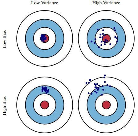
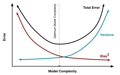
Bias-variance tradeoff
fig, (naive_ax, ips_ax) = plt.subplots(
    ncols=2, sharex=True, sharey=True,
    figsize=(2 * FIGURE_WIDTH, FIGURE_HEIGHT)
)

low, high = np.percentile(
    a_obs_rate,
    [100 * ALPHA / 2, 100 * (1 - ALPHA / 2)],
    axis=0
)

naive_ax.fill_between(
    plot_t, low, high,
    color=C[0], alpha=0.5
);
naive_ax.plot(
    plot_t, a_obs_rate.mean(axis=0),
    c=C[0]
);
naive_ax.hlines(
    A_RATE, 1, N,
    color=C[0], linestyles='--'
);

naive_ax.set_xlim(1, N);
naive_ax.set_xlabel("Sessions");

naive_ax.set_ylim(0., 3 * A_RATE);
naive_ax.yaxis.set_major_formatter(pct_formatter);
naive_ax.set_ylabel("Reward rate");

naive_ax.set_title("Naive estimate");

low, high = np.percentile(
    a_ips_est,
    [100 * ALPHA / 2, 100 * (1 - ALPHA / 2)],
    axis=0
)

ips_ax.fill_between(
    plot_t, low, high,
    color='k', alpha=0.5
);
ips_ax.plot(
    plot_t, a_ips_est.mean(axis=0),
    c='k'
);
ips_ax.hlines(
    A_RATE, 1, N,
    color=C[0], linestyles='--'
);

ips_ax.set_xlabel("Sessions");
ips_ax.set_title("IPS estimate");

fig.suptitle(f"Cumulative bandit performance ({N_BANDIT} simulations)");

fig
Intuition: the variant with the highest reward rate should receive the most traffic.
obs_opp_sign = np.sign(
    (a_obs_rate - b_obs_rate) \
        * ((arms == 0).cumsum(axis=1) - (arms == 1).cumsum(axis=1))
) == -1
ips_opp_sign = np.sign(
    (a_ips_est - b_ips_est) \
        * ((arms == 0).cumsum(axis=1) - (arms == 1).cumsum(axis=1))
) == -1
fig, ax = plt.subplots()

ax.plot(
    plot_t, obs_opp_sign.mean(axis=0),
    label="Naive estimate"
);
ax.plot(
    plot_t, ips_opp_sign.mean(axis=0),
    label="IPS estimate"
);

ax.set_xlim(1, N);
ax.set_xlabel("Sessions");

ax.yaxis.set_major_formatter(pct_formatter);
ax.set_ylabel("Probability intuition is wrong");

ax.legend(loc=1);

fig

%%bash
jupyter nbconvert \
    --to=slides \
    --reveal-prefix=https://cdnjs.cloudflare.com/ajax/libs/reveal.js/3.2.0/ \
    --output=data-philly-april-2018-bayes-bandits \
    ./Data\ Philly\ April\ 2018\ -\ Two\ Years\ of\ Bayesian\ Bandits\ for\ E-Commerce.ipynb
[NbConvertApp] Converting notebook ./Data Philly April 2018 - Two Years of Bayesian Bandits for E-Commerce.ipynb to slides
[NbConvertApp] Writing 2506844 bytes to ./data-philly-april-2018-bayes-bandits.slides.html