A Dockerfile that will produce a container with all the dependencies necessary to run this notebook is available here.

In [1]:

%matplotlib inline

In [2]:

import datetime
import logging
from warnings import filterwarnings

In [3]:

from matplotlib import pyplot as plt
from matplotlib.ticker import StrMethodFormatter
import numpy as np
import pandas as pd
import scipy as sp
import seaborn as sns
from sklearn.preprocessing import LabelEncoder
from theano import pprint

In [4]:

sns.set(color_codes=True)
pct_formatter = StrMethodFormatter('{x:.1%}')

In [5]:

# configure pyplot for readability when rendered as a slideshow and projected
FIG_WIDTH, FIG_HEIGHT = 8, 6
plt.rc('figure', figsize=(FIG_WIDTH, FIG_HEIGHT))

LABELSIZE = 14
plt.rc('axes', labelsize=LABELSIZE)
plt.rc('axes', titlesize=LABELSIZE)
plt.rc('figure', titlesize=LABELSIZE)
plt.rc('legend', fontsize=LABELSIZE)
plt.rc('xtick', labelsize=LABELSIZE)
plt.rc('ytick', labelsize=LABELSIZE)

In [6]:

filterwarnings('ignore', 'findfont')
filterwarnings('ignore', "Conversion of the second argument of issubdtype")
filterwarnings('ignore', "Set changed size during iteration")

# keep theano from complaining about compile locks for small models
(logging.getLogger('theano.gof.compilelock')
        .setLevel(logging.CRITICAL))

In [7]:

SEED = 54902 # from random.org, for reproducibility

np.random.seed(SEED)

The HMC Revolution is Open Source¶

Probabilistic Programming with PyMC3¶

@AustinRochford • Tom Tom AMLC • Charlottesville • 4/11/19¶

Who am I?¶

PyMC3 developer • Chief Data Scientist @ Monetate ¶

@AustinRochford • Website • GitHub ¶

arochford@monetate.com • austin.rochford@gmail.com ¶

About This Talk¶

Sorry, something went wrong. Reload?

Sorry, we cannot display this file.

Sorry, this file is invalid so it cannot be displayed.

view raw hmc-oss-pymc3-odsc-west-2018.ipynb hosted with ❤ by GitHub

About Monetate¶

Founded 2008, web optimization and personalization SaaS
Observed 5B impressions and $4.1B in revenue during Cyber Week 2017

monetate.com/about/careers

Modern Bayesian Inference¶

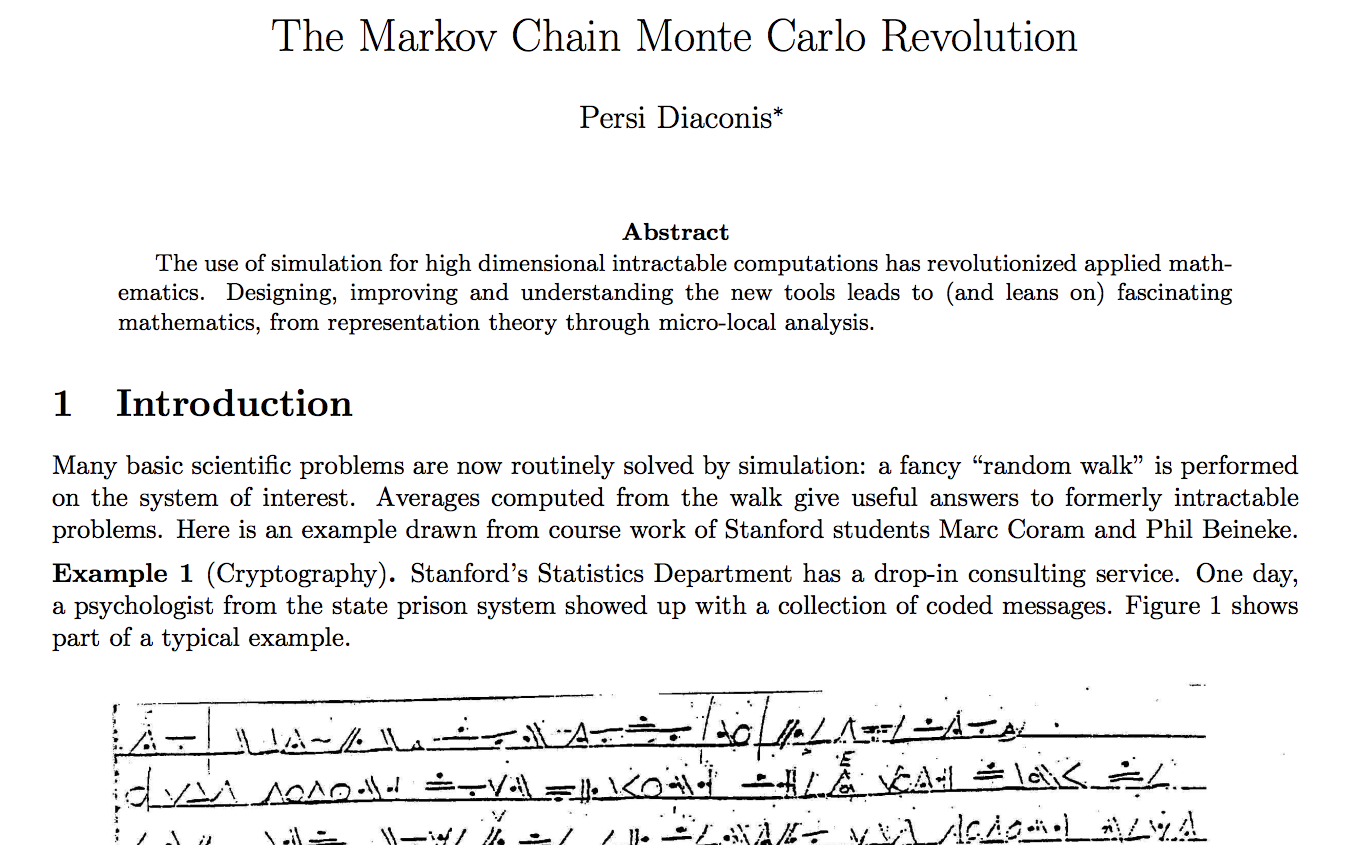
The Markov Chain Monte Carlo Revolution by famous probabilist Persi Diaconis gives an excellent overview of applications of simulation to many quantitative problems.

Motivating Examples¶

2017 UK General Election¶

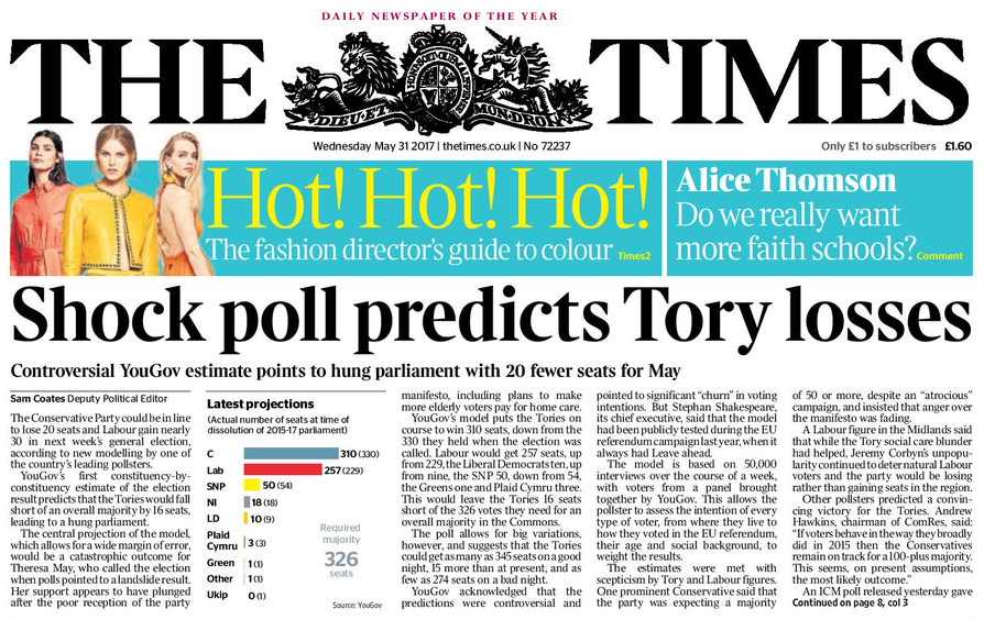
YouGov, a polling and opinion data company, correctly called a hung parilment as a result of the 2017 UK general elections in the UK using a Bayesian opinion modeling technique knowns as multilevel regression with poststratification (MRP) to produce accurate estimates of voter preferences in the UK's 650 parliamentary constituences.

Source

NBA Foul Calls¶

Source

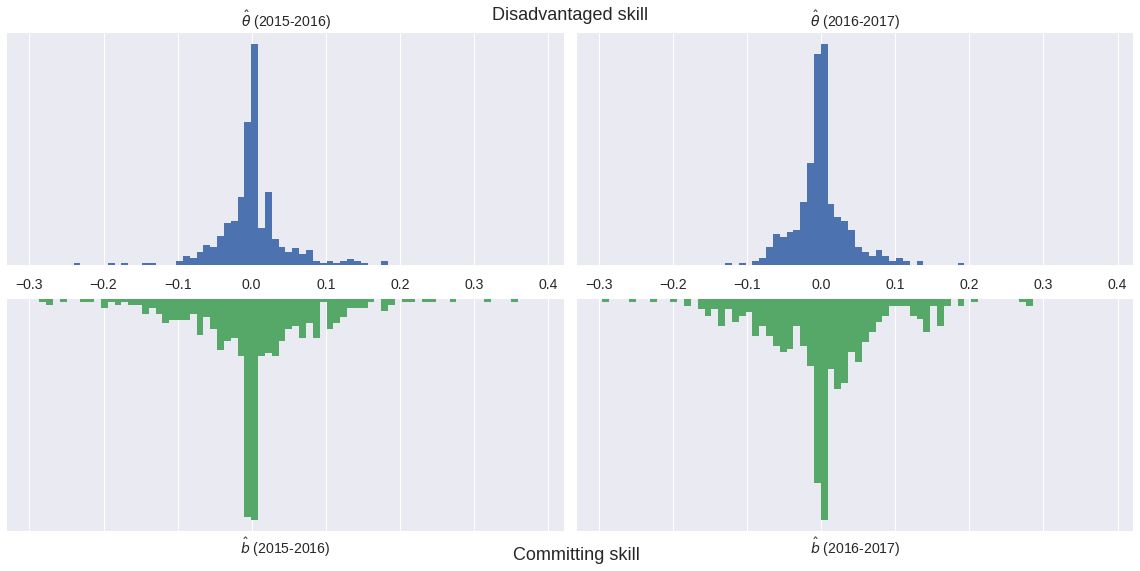
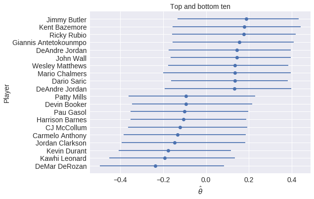
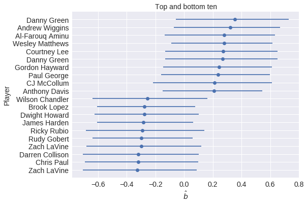
I have done some work using Bayesian methods to study whether or not committing/drawing fouls is a measurable skill among NBA players.

Player skills(?)¶

Probabilistic Programming¶

Data Science — inference enables storytelling¶

Probabilistic Programming — storytelling enables inference¶

The Monty Hall Problem¶

Initially, we have no information about which door the prize is behind.

In [8]:

import pymc3 as pm

with pm.Model() as monty_model:
    prize = pm.DiscreteUniform('prize', 0, 2)

If we choose door one:

	Monty can open
Prize behind	Door 1	Door 2	Door 3
Door 1	No	Yes	Yes
Door 2	No	No	Yes
Door 3	No	Yes	No

In [9]:

from theano import tensor as tt

with monty_model:
    p_open = pm.Deterministic(
        'p_open',
        tt.switch(tt.eq(prize, 0),
            np.array([0., 0.5, 0.5]), # it is behind the first door
        tt.switch(tt.eq(prize, 1),
            np.array([0., 0., 1.]),   # it is behind the second door
            np.array([0., 1., 0.])))  # it is behind the third door
    )

Monty opened the third door, revealing a goat.

In [10]:

with monty_model:
    opened = pm.Categorical('opened', p_open, observed=2)

Should we switch our choice of door?

In [11]:

CHAINS = 3

SAMPLE_KWARGS = {
    'chains': CHAINS,
    'cores': CHAINS,
    'random_seed': list(SEED + np.arange(CHAINS))
}

In [12]:

MONTY_SAMPLE_KWARGS = {
    'init': None,
    'compute_convergence_checks': False,
    **SAMPLE_KWARGS
}

In [13]:

with monty_model:
    monty_trace = pm.sample(1000, **MONTY_SAMPLE_KWARGS)
    
monty_df = pm.trace_to_dataframe(monty_trace)

Multiprocess sampling (3 chains in 3 jobs)
Metropolis: [prize]
Sampling 3 chains: 100%|██████████| 4500/4500 [00:01<00:00, 4173.25draws/s]

In [14]:

monty_df['prize'].head()

Out[14]:

0    0
1    0
2    0
3    0
4    1
Name: prize, dtype: int64

In [15]:

ax = (monty_df['prize']
              .value_counts(normalize=True, ascending=True)
              .plot(kind='bar', color='C0'))

ax.set_xlabel("Door");
ax.yaxis.set_major_formatter(pct_formatter);
ax.set_ylabel("Probability of prize");

From the PyMC3 documentation:

PyMC3 is a Python package for Bayesian statistical modeling and Probabilistic Machine Learning which focuses on advanced Markov chain Monte Carlo and variational fitting algorithms. Its flexibility and extensibility make it applicable to a large suite of problems.

Case Study: NBA Foul Calls¶

Question: Is (not) committing and/or drawing fouls a measurable player skill?

See this talk or this post for more information on the data, expanded models, and conclusions from this case study.

In [16]:

%%bash
DATA_URI=https://raw.githubusercontent.com/polygraph-cool/last-two-minute-report/32f1c43dfa06c2e7652cc51ea65758007f2a1a01/output/all_games.csv
DATA_DEST=/tmp/all_games.csv

if [[ ! -e $DATA_DEST ]];
then
    wget -q -O $DATA_DEST $DATA_URI
fi

In [17]:

USECOLS = [
    'period',
    'seconds_left',
    'call_type',
    'committing_player',
    'disadvantaged_player',
    'review_decision',
    'play_id',
    'away',
    'home',
    'date',
    'score_away',
    'score_home',
    'disadvantaged_team',
    'committing_team'
]

In [18]:

orig_df = pd.read_csv(
    '/tmp/all_games.csv',
    usecols=USECOLS,
    index_col='play_id',
    parse_dates=['date']
)

In [19]:

orig_df.head(n=2).T

Out[19]:

play_id	20150301CLEHOU-0	20150301CLEHOU-1
period	Q4	Q4
seconds_left	112	103
call_type	Foul: Shooting	Foul: Shooting
committing_player	Josh Smith	J.R. Smith
disadvantaged_player	Kevin Love	James Harden
review_decision	CNC	CC
away	CLE	CLE
home	HOU	HOU
date	2015-03-01 00:00:00	2015-03-01 00:00:00
score_away	103	103
score_home	105	105
disadvantaged_team	CLE	HOU
committing_team	HOU	CLE

In [20]:

foul_df = orig_df[
    orig_df.call_type
           .fillna("UNKNOWN")
           .str.startswith("Foul")
]

In [21]:

FOULS = [
    f"Foul: {foul_type}"
    for foul_type in [
        "Personal",
        "Shooting",
        "Offensive",
        "Loose Ball",
        "Away from Play"
    ]
]

In [22]:

TEAM_MAP = {
    "NKY": "NYK",
    "COS": "BOS",
    "SAT": "SAS",
    "CHi": "CHI",
    "LA)": "LAC",
    "AT)": "ATL",
    "ARL": "ATL"
}

def correct_team_name(col):
    def _correct_team_name(df):
        return df[col].apply(lambda team_name: TEAM_MAP.get(team_name, team_name))
    
    return _correct_team_name

In [23]:

def date_to_season(date):
    if date >= datetime.datetime(2017, 10, 17):
        return '2017-2018'
    elif date >= datetime.datetime(2016, 10, 25):
        return '2016-2017'
    elif date >= datetime.datetime(2015, 10, 27):
        return '2015-2016'
    else:
        return '2014-2015'

In [24]:

clean_df = (foul_df.where(lambda df: df.period == "Q4")
                   .where(lambda df: (df.date.between(datetime.datetime(2016, 10, 25),
                                                      datetime.datetime(2017, 4, 12))
                                      | df.date.between(datetime.datetime(2015, 10, 27),
                                                       datetime.datetime(2016, 5, 30)))
                         )
                   .assign(
                       review_decision=lambda df: df.review_decision.fillna("INC"),
                       committing_team=correct_team_name('committing_team'),
                       disadvantged_team=correct_team_name('disadvantaged_team'),
                       away=correct_team_name('away'),
                       home=correct_team_name('home'),
                       season=lambda df: df.date.apply(date_to_season)
                    )
                   .where(lambda df: df.call_type.isin(FOULS))
                   .dropna()
                   .drop('period', axis=1)
                   .assign(call_type=lambda df: (df.call_type
                                                   .str.split(': ', expand=True)  
                                                   .iloc[:, 1])))

In [25]:

player_enc = LabelEncoder().fit(
    np.concatenate((
        clean_df.committing_player,
        clean_df.disadvantaged_player
    ))
)
n_player = player_enc.classes_.size

season_enc = LabelEncoder().fit(
    clean_df.season
)
n_season = season_enc.classes_.size

In [26]:

df = (clean_df[['seconds_left']]
              .round(0)
              .assign(
                foul_called=1. * clean_df.review_decision.isin(['CC', 'INC']),
                player_committing=player_enc.transform(clean_df.committing_player),
                player_disadvantaged=player_enc.transform(clean_df.disadvantaged_player),
                score_committing=clean_df.score_home.where(
                    clean_df.committing_team == clean_df.home,
                    clean_df.score_away
                ),
                score_disadvantaged=clean_df.score_home.where(
                    clean_df.disadvantaged_team == clean_df.home,
                    clean_df.score_away
                ),
                season=season_enc.transform(clean_df.season)
              ))

In [27]:

player_committing = df.player_committing.values
player_disadvantaged = df.player_disadvantaged.values

season = df.season.values

In [28]:

def hierarchical_normal(name, shape):
    Δ = pm.Normal(f'Δ_{name}', 0., 1., shape=shape)
    σ = pm.HalfNormal(f'σ_{name}', 5.)
    
    return pm.Deterministic(name, Δ * σ)

Model outline¶

$\operatorname{log-odds}(\textrm{Foul}) \ \sim \textrm{Season factor} + \left(\textrm{Disadvantaged skill} - \textrm{Committing skill}\right)$

In [29]:

with pm.Model() as irt_model:
    β_season = pm.Normal('β_season', 0., 2.5, shape=n_season)
    
    θ = hierarchical_normal('θ', n_player) # disadvantaged skill
    b = hierarchical_normal('b', n_player) # committing skill

    p = pm.math.sigmoid(
        β_season[season] + θ[player_disadvantaged] - b[player_committing]
    )
    
    obs = pm.Bernoulli(
        'obs', p,
        observed=df['foul_called'].values
    )

Metropolis-Hastings Inference¶

In [30]:

with irt_model: 
    step = pm.Metropolis()
    met_trace = pm.sample(5000, step=step, **SAMPLE_KWARGS)

Multiprocess sampling (3 chains in 3 jobs)
CompoundStep
>Metropolis: [σ_b]
>Metropolis: [Δ_b]
>Metropolis: [σ_θ]
>Metropolis: [Δ_θ]
>Metropolis: [β_season]
Sampling 3 chains: 100%|██████████| 16500/16500 [01:48<00:00, 152.44draws/s]
The gelman-rubin statistic is larger than 1.4 for some parameters. The sampler did not converge.
The estimated number of effective samples is smaller than 200 for some parameters.

In [31]:

met_gr_stats = pm.gelman_rubin(met_trace)
met_θ_worst_ix = met_gr_stats['θ'].argmax()
met_θ_worst = np.concatenate([
    chain_values[np.newaxis, :, met_θ_worst_ix]
        for chain_values in met_trace.get_values('θ', combine=False)
])

In [32]:

trace_fig, (trace_ax, hist_ax) = plt.subplots(ncols=2, figsize=(16, 6))

trace_ax.plot(met_θ_worst.T, alpha=0.5);

trace_ax.set_xticklabels([]);
trace_ax.set_xlabel("Sample index");

worst_param_label = r"$\theta_{" + str(met_θ_worst_ix) + "}$"

trace_ax.set_ylabel(worst_param_label);

sns.distplot(
    met_trace['θ'][:, met_θ_worst_ix],
    kde=False, norm_hist=True, ax=hist_ax
);

hist_ax.set_xlabel(worst_param_label);

hist_ax.set_yticks([]);
hist_ax.set_ylabel("Posterior density");

trace_fig.suptitle("Metropolis-Hastings");

/opt/conda/lib/python3.6/site-packages/matplotlib/axes/_axes.py:6521: MatplotlibDeprecationWarning: 
The 'normed' kwarg was deprecated in Matplotlib 2.1 and will be removed in 3.1. Use 'density' instead.
  alternative="'density'", removal="3.1")

In [33]:

trace_fig

Out[33]:

In [34]:

max(np.max(var_stats) for var_stats in pm.gelman_rubin(met_trace).values())

Out[34]:

3.1038666861280597

The Curse of Dimensionality¶

This model has

In [35]:

n_param = n_season + 2 * n_player
n_param

Out[35]:

parameters

The curse of dimensionality is a well-known concept in machine learning. It refers to the fact that as the number of dimensions in the sample space increases, samples become (on average) far apart quite quickly. It is related to the more complicated phenomenon of concentration of measure, which is the actual motivation for Hamiltonian Monte Carlo (HMC) algorithms.

The following plot illustrates one of the one aspect of the curse of dimensionality, that the volume of the unit ball tends to zero as the dimensionality of the space becomes large. That is, if

$\begin{align*} S_d & = \left\{\left.\vec{x} \in \mathbb{R}^d\ \right|\ x_1^2 + \cdots + x_d^2 \leq 1\right\}, \\ \operatorname{Vol}(S_d) & = \frac{2 \pi^{\frac{d}{2}}}{d\ \Gamma\left(\frac{d}{2}\right)}. \end{align*}$

And we get that $\operatorname{Vol}(S_d) \to 0$ as $d \to \infty$ .

In [36]:

def sphere_volume(d):
    return 2. * np.power(np.pi, d / 2.) / d / sp.special.gamma(d / 2)

In [37]:

fig, ax = plt.subplots()

d_plot = np.linspace(1, n_param)

ax.plot(d_plot, sphere_volume(d_plot));

ax.set_xscale('log');
ax.set_xlabel("Dimensions");

ax.set_yscale('log');
ax.set_ylabel("Volume of the unit sphere");

In [38]:

fig

Out[38]:

Hamiltonian Monte Carlo Inference¶

Bayesian inference ⇔ Differential geometry¶

Case Study Continued: NBA Foul Calls¶

In [39]:

with irt_model:
    nuts_trace = pm.sample(500, **SAMPLE_KWARGS)

Auto-assigning NUTS sampler...
Initializing NUTS using jitter+adapt_diag...
Multiprocess sampling (3 chains in 3 jobs)
NUTS: [σ_b, Δ_b, σ_θ, Δ_θ, β_season]
Sampling 3 chains: 100%|██████████| 3000/3000 [02:14<00:00, 22.23draws/s]

In [40]:

nuts_gr_stats = pm.gelman_rubin(nuts_trace)
max(np.max(var_stats) for var_stats in nuts_gr_stats.values())

Out[40]:

1.0069298341016355

In [41]:

nuts_θ_worst = np.concatenate([
    chain_values[np.newaxis, :, met_gr_stats['θ'].argmax()]
        for chain_values in nuts_trace.get_values('θ', combine=False)
])

In [42]:

fig, (met_axs, nuts_axs)  = plt.subplots(nrows=2, ncols=2, figsize=(16, 12))

(met_trace_ax, met_hist_ax) = met_axs

met_trace_ax.plot(met_θ_worst.T, alpha=0.5);

worst_param_label = r"$\theta_{" + str(met_θ_worst_ix) + "}$"

met_trace_ax.set_ylabel("Metropolis-Hastings\n" + worst_param_label);

sns.distplot(
    met_trace['θ'][:, met_θ_worst_ix],
    kde=False, norm_hist=True, ax=met_hist_ax
);

XMIN = min(met_trace['θ'][:, met_θ_worst_ix].min(),
           nuts_trace['θ'][:, met_θ_worst_ix].min())
XMAX = min(met_trace['θ'][:, met_θ_worst_ix].max(),
           nuts_trace['θ'][:, met_θ_worst_ix].max())

met_hist_ax.set_xlim(XMIN, XMAX);

met_hist_ax.set_yticks([]);
met_hist_ax.set_ylabel("Posterior density");

(nuts_trace_ax, nuts_hist_ax) = nuts_axs

nuts_trace_ax.plot(nuts_θ_worst.T, alpha=0.5);

nuts_trace_ax.set_xlabel("Sample index");

nuts_trace_ax.set_ylabel("HMC\n" + worst_param_label);

sns.distplot(
    nuts_trace['θ'][:, met_θ_worst_ix],
    kde=False, norm_hist=True, ax=nuts_hist_ax
);

nuts_hist_ax.set_xlim(XMIN, XMAX);
nuts_hist_ax.set_xlabel(worst_param_label);

nuts_hist_ax.set_yticks([]);
nuts_hist_ax.set_ylabel("Posterior density");

fig.tight_layout();

/opt/conda/lib/python3.6/site-packages/matplotlib/axes/_axes.py:6521: MatplotlibDeprecationWarning: 
The 'normed' kwarg was deprecated in Matplotlib 2.1 and will be removed in 3.1. Use 'density' instead.
  alternative="'density'", removal="3.1")

In [43]:

fig

Out[43]:

Basketball strategy leads to more complexity¶

In [44]:

df['trailing_committing'] = (df.score_committing
                               .lt(df.score_disadvantaged)
                               .mul(1.)
                               .astype(np.int64))

In [45]:

def make_foul_rate_yaxis(ax, label="Observed foul call rate"):
    ax.yaxis.set_major_formatter(pct_formatter)
    ax.set_ylabel(label)
    
    return ax

In [46]:

def make_time_axes(ax,
                   xlabel="Seconds remaining in game",
                   ylabel="Observed foul call rate"):
    ax.invert_xaxis()
    ax.set_xlabel(xlabel)
    
    return make_foul_rate_yaxis(ax, label=ylabel)

In [47]:

fig = make_time_axes(
    df.pivot_table('foul_called', 'seconds_left', 'trailing_committing')
      .rolling(20).mean()
      .rename(columns={0: "No", 1: "Yes"})
      .rename_axis("Committing team is trailing", axis=1)
      .plot()
).figure

In [48]:

fig

Out[48]:

Next Steps with Probabilistic Programming¶

The following books/GitHub repositories provide good introductions to PyMC3 and Bayesian statistics.

PyMC3¶

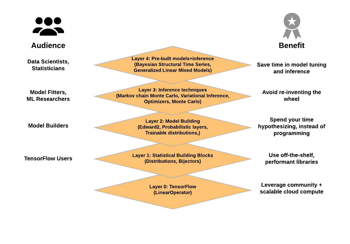
Probabilistic Programming Ecosystem¶

PyMC4?¶

TensorFlow Probability

Prototype repository

Hamiltonian Monte Carlo¶

A Conceptual Introduction to Hamiltonian Monte Carlo

Thank you!¶