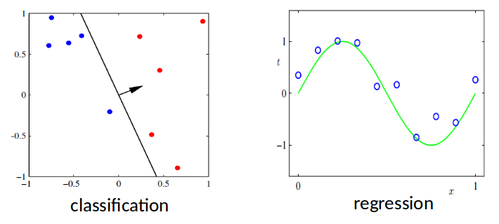
Supervised Learning¶
- Goal
- Given data X in feature sapce and the labels Y
- Learn to predict Y from X
- Labels could be discrete or continuous
- Discrete-valued labels: Classification
- Continuous-valued labels: Regression
Notation¶
- In this lecture, we will use
- Let vector →xn∈\RD denote the nth data. D denotes number of attributes in dataset.
- Let vector ϕ(→xn)∈\RM denote features for data →xn. ϕj(→xn) denotes the jth feature for data xn.
- Feature ϕ(→xn) is the artificial features which represents the preprocessing step. ϕ(→xn) is usually some combination of transformations of →xn. For example, ϕ(→x) could be vector constructed by [→xTn,cos(→xn)T,exp(→xn)T]T. If we do nothing to →xn, then ϕ(→xn)=→xn.
- Continuous-valued label vector t∈\RD (target values). tn∈\R denotes the target value for ith data.
Notation: Example¶
- The table below is a dataset describing acceleration of the aircraft along a runway. Based on our notations above, we have D=7. Regardless of the header row, target value t is the first column and xn denote the data on the nth row, 2th to 7th columns.
- We could manipulate the data to have our own features. For example,
- If we only choose the first three attributes as features, i.e. ϕ(→xn)=→xn[1:3], then M=3
- If we let ϕ(→xn)=[→xTn,cos(→xn)T,exp(→xn)T], then M=3×D=21
- We could also let ϕ(→xn)=→xn, then M=D=7. This will occur frequently in later lectures.

(Example taken from [here](http://www.flightdatacommunity.com/linear-regression-applied-to-take-off/))
Linear Regression¶
Linear Regression (1D Inputs)¶
- Consider 1D case (i.e. D=1)
- Given a set of observations x1,…,xN∈\RM
- and corresponding target values t1,…,tN
- We want to learn a function y(xn,→w)≈tn to predict future values.
of which feature coefficient →w=[w0,w1,w2,…,wM−1]T, feature ϕ(xn)=[1,xn,x2n,…,xM−1n] (here we add a bias term ϕ0(xn)=1 to features).
Regression: Noisy Data¶
In [2]:
regression_example_draw(degree1=0,degree2=1,degree3=3, ifprint=True)

The expression for the first polynomial is y=-0.129
The expression for the second polynomial is y=-0.231+0.598x^1
The expression for the third polynomial is y=0.085-0.781x^1+1.584x^2-0.097x^3
Basis Functions¶
- For feature basis function, we used polynomial functions for example above.
- In fact, we have multiple choices for basis function ϕj(→x).
- Different basis functions will produce different features, thus may have different performances in prediction.
In [3]:
basis_function_plot()

Linear Regression (General Case)¶
- The function y(→xn,→w) is linear in parameters →w.
- Goal: Find the best value for the weights →w.
- For simplicity, add a bias term ϕ0(→xn)=1.
of which ϕ(→xn)=[ϕ0(→xn),ϕ1(→xn),ϕ2(→xn),…,ϕM−1(→xn)]T
Least Squares¶
Least Squares: Objective Function¶
- We will find the solution →w to linear regression by minimizing a cost/objective function.
- When the objective function is sum of squared errors (sum differences between target t and prediction y over entire training data), this approach is also called least squares.
- The objective function is

How to Minimize the Objective Function?¶
- We will solve the least square problem in two approaches:
- Gradient Descent Method: approach the solution step by step. We will show two ways when iterate:
- Batch Gradient Descent
- Stochastic Gradient Descent
- Closed Form Solution
- Gradient Descent Method: approach the solution step by step. We will show two ways when iterate:
Method I: Gradient Descent—Gradient Calculation¶
- To minimize the objective function, take derivative w.r.t coefficient vector →w:
- Since we are taking derivative of a scalar E(→w) w.r.t a vector →w, the derivative ∇→wE(→w) will be a vector.
- For details about matrix/vector derivative, please refer to appendix attached in the end of the slide.
Method I-1: Gradient Descent—Batch Gradient Descent¶
- Input: Given dataset {(→xn,tn)}Nn=1
- Initialize: →w0, learning rate η
- Repeat until convergence:
- ∇→wE(→wold)=∑Nn=1(→wToldϕ(→xn)−tn)ϕ(→xn)
- →wnew=→wold−η∇→wE(→wold)
- End
- Output: →wfinal
Method I-2: Gradient Descent—Stochastic Gradient Descent¶
Main Idea: Instead of computing batch gradient (over entire training data), just compute gradient for individual training sample and update.
- Input: Given dataset {(→xn,tn)}Nn=1
- Initialize: →w0, learning rate η
- Repeat until convergence:
- Random shuffle {(→xn,tn)}Nn=1
- For n=1,…,N do:
- ∇→wE(→wold|→xn)=(→wToldϕ(→xn)−tn)ϕ(→xn)
- →wnew=→wold−η∇→wE(→wold|→xn)
- End
- End
- Output: →wfinal
Method II: Closed Form Solution¶
Main Idea: Compute gradient and set to gradient to zero, solving in closed form.
- Objective Function E(→w)=12∑Nn=1(→wTϕ(→xn)−tn)2=12∑Nn=1(ϕ(→xn)T→w−tn)2
- Let →e=[ϕ(→x1)T→w−t1,ϕ(→x2)T→w−t2,…,ϕ(→xN)T→w−tN]T, we have E(→w)=12→eT→e=12∥→e ∥2
- Look at →e:
Here Φ∈\RN×M is called design matrix. Each row represents one sample. Each column represents one feature Φ=[ϕ(→x1)Tϕ(→x2)T⋮ϕ(→xN)T]=[ϕ0(→x1)ϕ1(→x1)⋯ϕM−1(→x1)ϕ0(→x2)ϕ1(→x2)⋯ϕM−1(→x2)⋮⋮⋱⋮ϕ0(→xN)ϕ1(→xN)⋯ϕM−1(→xN)]
- From E(→w)=12‖→e‖2=12→eT→e and →e=Φ→w−→t, we have
- So the derivative is ∇→wE(→w)=ΦTΦ→w−ΦT→t
- To minimize E(→w), we need to let ∇→wE(→w)=ΦTΦ→w−ΦT→t=0, which is also ΦTΦ→w=ΦT→t
- When ΦTΦ is invertible (Φ has linearly independent columns), we simply have
of which Φ† is called the Moore-Penrose Pseudoinverse of Φ.
- We will talk about case ΦTΦ is non-invertible later.
Digression: Moore-Penrose Pseudoinverse¶
- When we have a matrix A that is non-invertible or not even square, we might want to invert anyway
- For these situations we use A†, the Moore-Penrose Pseudoinverse of A
- In general, we can get A† by SVD: if we write A∈\Rm×n=Um×mΣm×nVTn×n then A†∈\Rn×m=VΣ†UT, where Σ†∈\Rn×m is obtained by taking reciprocals of non-zero entries of ΣT.
- Particularly, when A has linearly independent columns then A†=(ATA)−1AT. When A is invertible, then A†=A−1.
Back to Closed Form Solution¶
- From previous derivation, we have ˆw=(ΦTΦ)−1ΦT→t≜Φ†→t.
- What if ΦTΦ is non-invertible? This corresponds to the case where Φ doesn't have linearly independent columns. For dataset, this means the feature vector of certain sample is the linear combination of feature vectors of some other samples.
- We could still resolve this using pseudoinverse.
- To make ∇→wE(→w)=ΦTΦ→w−ΦT→t=0, we have
of which (ΦTΦ)†ΦT=Φ†. This is left as an exercise. (Hint: use SVD)
- Now we could conclude the optimal →w in the sense that minimizes sum of squared errors is ˆ→w=Φ†→t
EECS 545: Machine Learning Lecture 04: Linear Regression I Instructor: Jacob Abernethy Date: January 20, 2015 Lecture Exposition Credit: Benjamin Bray