Lesson Outline
- Motivation
- Qualitative Approaches
- Thresholding
- Other types of images
- Selecting a good threshold
- Implementation
- Morphology
- Contouring / Mask Creation
Applications
- Simple two-phase materials (bone, cells, etc)
- Beyond 1 channel of depth
- Multiple phase materials
- Filling holes in materials
- Segmenting Fossils
- Attempting to segment the cortex in brain imaging

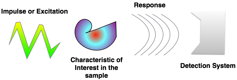
Motivation: Why do we do imaging experiments?
- Exploratory
- To visually, qualitatively examine samples and differences between them
- No prior knowledge or expectations
- To test a hypothesis
- Quantitative assessment coupled with statistical analysis
- Does temperature affect bubble size?
- Is this gene important for cell shape and thus mechanosensation in bone?
- Does higher canal volume make bones weaker?
- Does the granule shape affect battery life expectancy?
- What we are looking at

- What we get from the imaging modality
%matplotlib inline
from skimage.io import imread
from skimage.color import rgb2gray
import matplotlib.pyplot as plt
dkimg = imread("../common/figures/Average_prokaryote_cell.jpg")
plt.matshow(rgb2gray(dkimg), cmap = 'bone')
<matplotlib.image.AxesImage at 0x11f135c50>


Why do we perform segmentation?
- In model-based analysis every step we peform, simple or complicated is related to an underlying model of the system we are dealing with
- Occam's Razor is very important here : The simplest solution is usually the right one
- Bayesian, neural networks optimized using genetic algorithms with Fuzzy logic has a much larger parameter space to explore, establish sensitivity in, and must perform much better and be tested much more thoroughly than thresholding to be justified.
- We will cover some of these techniques in the next 2 lectures since they can be very powerful particularly with unknown data
Review: Filtering and Image Enhancement
- This was a noise process which was added to otherwise clean imaging data
- $$ I_{measured}(x,y) = I_{sample}(x,y) + \text{Noise}(x,y) $$
- What would the perfect filter be
- $$ \textit{Filter} \ast I_{sample}(x,y) = I_{sample}(x,y) $$
- $$ \textit{Filter} \ast \text{Noise}(x,y) = 0 $$
- $$ \textit{Filter} \ast I_{measured}(x,y) = \textit{Filter} \ast I_{real}(x,y) + \textit{Filter}\ast \text{Noise}(x,y) \rightarrow \bf I_{sample}(x,y) $$
- What most filters end up doing
- What bad filters do
Qualitative Metrics: What did people used to do?
- What comes out of our detector / enhancement process
%matplotlib inline
from skimage.io import imread
from skimage.color import rgb2gray
import matplotlib.pyplot as plt
dkimg = rgb2gray(imread("../common/figures/Average_prokaryote_cell.jpg"))
fig, (ax_hist, ax_img) = plt.subplots(1, 2, figsize = (12,6))
ax_hist.hist(dkimg.ravel())
ax_hist.set_xlabel('Absorption Coefficient')
ax_hist.set_ylabel('Pixel Count')
m_show_obj = ax_img.matshow(dkimg, cmap = 'bone')
cb_obj = plt.colorbar(m_show_obj)
cb_obj.set_label('Absorption Coefficient')

- Identify objects by eye
- Count, describe qualitatively: "many little cilia on surface", "long curly flaggelum", "elongated nuclear structure"
- Morphometrics
- Trace the outline of the object (or sub-structures)
- Can calculate the area by using equal-weight-paper
- Employing the "cut-and-weigh" method

Model-based Analysis
- Many different imaging modalities ( $\mu \textrm{CT}$ to MRI to Confocal to Light-field to AFM).
- Similarities in underlying equations
- different coefficients, units, and mechanism
Direct Imaging (simple)
In many setups there is un-even illumination caused by incorrectly adjusted equipment and fluctations in power and setups
- $F_{system}(a,b) = a*b$
- $I_{stimulus} = \textrm{Beam}_{profile}$
- $S_{system} = \alpha(\vec{x})$
$\longrightarrow \alpha(\vec{x})=\frac{I_{measured}(\vec{x})}{\textrm{Beam}_{profile}(\vec{x})}$
%matplotlib inline
from skimage.io import imread
from skimage.color import rgb2gray
import matplotlib.pyplot as plt
from skimage.morphology import disk
from scipy.ndimage import zoom
import numpy as np
cell_img = 1-rgb2gray(imread("../common/figures/Average_prokaryote_cell.jpg"))
s_beam_img = np.pad(disk(2)/1.0, [[1,1], [1,1]], mode = 'constant', constant_values = 0.2)
beam_img = zoom(s_beam_img,
[cell_img.shape[0]/7.0, cell_img.shape[1]/7.0])
fig, (ax_beam, ax_img, ax_det) = plt.subplots(1, 3, figsize = (12,4))
ax_beam.imshow(beam_img,
cmap = 'hot')
ax_beam.set_title('Beam Profile')
ax_img.imshow(cell_img,
cmap = 'hot')
ax_img.set_title('Sample Profile')
ax_det.imshow(cell_img*beam_img,
cmap = 'hot')
ax_det.set_title('Detector');

fig, (ax_prof) = plt.subplots(1, 1, figsize = (12,4))
ax_prof.plot(beam_img[beam_img.shape[0]//2], label = 'Beam Profile')
ax_prof.plot(cell_img[beam_img.shape[0]//2], label = 'Sample Image')
ax_prof.plot((cell_img*beam_img)[beam_img.shape[0]//2], label = 'Detector')
ax_prof.set_ylabel('Intensity')
ax_prof.set_xlabel('Pixel Position')
# make an interactive plot
import plotly.offline as py
import plotly.tools as tls
py.init_notebook_mode()
py.iplot(tls.mpl_to_plotly(fig))
Frequently there is a fall-off of the beam away from the center (as is the case of a Gaussian beam which frequently shows up for laser systems). This can make extracting detail away from the center challenging
fig, ax1 = plt.subplots(1,1, figsize = (8,8))
ax1.matshow(cell_img*beam_img,
cmap = 'hot');

Absorption Imaging (X-ray, Ultrasound, Optical)
- For absorption/attenuation imaging $\rightarrow$ Beer-Lambert Law
$$ I_{detector} = \underbrace{I_{source}}_{I_{stimulus}}\underbrace{\exp(-\alpha d)}_{S_{sample}} $$
- Different components have a different $\alpha$ based on the strength of the interaction between the light and the chemical / nuclear structure of the material
- For segmentation this model is:
- there are 2 (or more) distinct components that make up the image
- these components are distinguishable by their values (or vectors, colors, tensors, ...)
%matplotlib inline
import matplotlib.pyplot as plt
import numpy as np
import pandas as pd
I_source = 1.0
d = 1.0
alpha_1 = np.random.normal(1, 0.25, size = 100)
alpha_2 = np.random.normal(2, 0.25, size = 100)
alpha_3 = np.random.normal(3, 0.5, size = 100)
abs_df = pd.DataFrame([dict(alpha = c_x, material = c_mat) for c_vec, c_mat in zip([alpha_1, alpha_2, alpha_3],
['material 1', 'material 2', 'material 3']) for c_x in c_vec])
abs_df['I_detector'] = I_source*np.exp(-abs_df['alpha']*d)
fig, ((ax1, ax2), (ax3, ax4)) = plt.subplots(2,2, figsize = (12, 8))
for c_mat, c_df in abs_df.groupby('material'):
ax1.scatter(x = c_df['alpha'],
y = c_df['I_detector'],
label = c_mat)
ax3.hist(c_df['alpha'], alpha = 0.5, label = c_mat)
ax2.hist(c_df['I_detector'], alpha = 0.5, label = c_mat, orientation="horizontal")
ax1.set_xlabel('$\\alpha(x,y)$', fontsize = 15)
ax1.set_ylabel('$I_{detector}$', fontsize = 18)
ax1.legend()
ax2.legend()
ax3.legend(loc = 0)
ax4.axis('off');

Example Mammography
Mammographic imaging is an area where model-based absorption imaging is problematic. Even if we assume a constant illumination (rarely the case),
$$ I_{detector} = \underbrace{I_{source}}_{I_{stimulus}}\underbrace{\exp(-\alpha d)}_{S_{sample}} $$$$ \downarrow $$$$ I_{detector} = \exp(-\alpha(x,y) d(x,y)) $$$$ \downarrow $$$$ I_{detector} = \exp(-\int_{0}^{l}\alpha(x,y, z) dz) $$Specifically the problem is related to the inability to separate the $\alpha$ and $d$ terms. We model a basic breast volume as a half sphere with a constant absorption factor.
$$\alpha(x,y,z) = 1e-2$$The $\int$ then turns into a $\Sigma$ in discrete space
%matplotlib inline
import matplotlib.pyplot as plt
import numpy as np
from skimage.morphology import ball
breast_mask = ball(50)[:,50:]
# just for 3d rendering, don't worry about it
import plotly.offline as py
from plotly.figure_factory import create_trisurf
py.init_notebook_mode()
from skimage.measure import marching_cubes_lewiner
vertices, simplices, _, _ = marching_cubes_lewiner(breast_mask>0)
x,y,z = zip(*vertices)
fig = create_trisurf(x=x,
y=y,
z=z,
plot_edges=False,
simplices=simplices,
title="Breast Phantom")
py.iplot(fig)
breast_alpha = 1e-2
breast_vol = breast_alpha*breast_mask
i_detector = np.exp(-np.sum(breast_vol,2))
fig, (ax_hist, ax_breast) = plt.subplots(1, 2, figsize = (20,8))
b_img_obj = ax_breast.imshow(i_detector, cmap = 'bone_r')
plt.colorbar(b_img_obj)
ax_hist.hist(i_detector.flatten())
ax_hist.set_xlabel('$I_{detector}$')
ax_hist.set_ylabel('Pixel Count');

If we know that $\alpha$ is constant we can reconstruct d from the image
breast_thickness = -np.log(i_detector)/breast_alpha
fig, (ax_hist, ax_breast) = plt.subplots(1, 2, figsize = (12,5))
b_img_obj = ax_breast.imshow(breast_thickness, cmap = 'bone')
plt.colorbar(b_img_obj)
ax_hist.hist(breast_thickness.flatten())
ax_hist.set_xlabel('Breast Thickness ($d$)\nIn Pixels')
ax_hist.set_ylabel('Pixel Count');

from mpl_toolkits.mplot3d import Axes3D
fig = plt.figure(figsize = (8, 4), dpi = 200)
ax = fig.gca(projection='3d')
# Plot the surface.
yy, xx = np.meshgrid(np.linspace(0, 1, breast_thickness.shape[1]),
np.linspace(0, 1, breast_thickness.shape[0]))
surf = ax.plot_surface(xx, yy, breast_thickness, cmap=plt.cm.jet,
linewidth=0, antialiased=False)
ax.view_init(elev = 30, azim = 45)
ax.set_zlabel('Breast Thickness');

We run into problems when the $\alpha$ is no longer constant. For example if we place a dark lump in the center of the breast. It is impossible to tell if the breast if thicker or if the lump inside is denser. For the lump below we can see on the individual slices of the sample that the lesion appears quite clearly and is very strangely shaped.
breast_vol = breast_alpha*breast_mask
renorm_slice = np.sum(breast_mask[10:40, 0:25], 2)/np.sum(breast_mask[30, 10])
breast_vol[10:40, 0:25] /= np.stack([renorm_slice]*breast_vol.shape[2],-1)
from skimage.util import montage as montage2d
fig, ax1 = plt.subplots(1,1, figsize = (12, 12))
ax1.imshow(montage2d(breast_vol.swapaxes(0,2).swapaxes(1,2)[::3]),
cmap = 'bone', vmin = breast_alpha*.8, vmax = breast_alpha*1.2)
<matplotlib.image.AxesImage at 0x11ecfcf28>

When we make the projection and apply Beer's Law we see that it appears as a relatively constant region in the image
i_detector = np.exp(-np.sum(breast_vol,2))
fig, (ax_hist, ax_breast) = plt.subplots(1, 2, figsize = (20,8))
b_img_obj = ax_breast.imshow(i_detector, cmap = 'bone_r')
plt.colorbar(b_img_obj)
ax_hist.hist(i_detector.flatten())
ax_hist.set_xlabel('$I_{detector}$')
ax_hist.set_ylabel('Pixel Count');

And as a flat constant region in the thickness reconstruction. So we fundamentally from this single image cannot answer is the breast oddly shaped or does it have an possible tumor inside of it
breast_thickness = -np.log(i_detector)/1e-2
fig, (ax_hist, ax_breast) = plt.subplots(1, 2, figsize = (12,5))
b_img_obj = ax_breast.imshow(breast_thickness, cmap = 'bone')
plt.colorbar(b_img_obj)
ax_hist.hist(breast_thickness.flatten())
ax_hist.set_xlabel('Breast Thickness ($d$)\nIn Pixels')
ax_hist.set_ylabel('Pixel Count');

from mpl_toolkits.mplot3d import Axes3D
fig = plt.figure(figsize = (8, 4), dpi = 200)
ax = fig.gca(projection='3d')
# Plot the surface.
yy, xx = np.meshgrid(np.linspace(0, 1, breast_thickness.shape[1]),
np.linspace(0, 1, breast_thickness.shape[0]))
surf = ax.plot_surface(xx, yy, breast_thickness, cmap=plt.cm.jet,
linewidth=0, antialiased=False)
ax.view_init(elev = 30, azim = 130)
ax.set_zlabel('Breast Thickness');

Where does segmentation get us?
We convert a decimal value (or something even more complicated like 3 values for RGB images, a spectrum for hyperspectral imaging, or a vector / tensor in a mechanical stress field)
to a single, discrete value (usually true or false, but for images with phases it would be each phase, e.g. bone, air, cellular tissue)
2560 x 2560 x 2160 x 32 bit = 56GB / sample
- 2560 x 2560 x 2160 x 1 bit = 1.75GB / sample
Applying a threshold to an image
Start out with a simple image of a cross with added noise $$ I(x,y) = f(x,y) $$
%matplotlib inline
import matplotlib.pyplot as plt
import numpy as np
import pandas as pd
nx = 5
ny = 5
xx, yy = np.meshgrid(np.arange(-nx, nx+1)/nx*2*np.pi,
np.arange(-ny, ny+1)/ny*2*np.pi)
cross_im = 1.5*np.abs(np.cos(xx*yy))/(np.abs(xx*yy)+(3*np.pi/nx))+np.random.uniform(-0.25, 0.25, size = xx.shape)
plt.matshow(cross_im, cmap = 'hot')
plt.colorbar()
<matplotlib.colorbar.Colorbar at 0x10aa79898>

The intensity can be described with a probability density function $$ P_f(x,y) $$
fig, ax1 = plt.subplots(1,1)
ax1.hist(cross_im.ravel(), 20)
ax1.set_title('$P_f(x,y)$')
ax1.set_xlabel('Intensity')
ax1.set_ylabel('Pixel Count');

Applying a threshold to an image
By examining the image and probability distribution function, we can deduce that the underyling model is a whitish phase that makes up the cross and the darkish background
Applying the threshold is a deceptively simple operation
$$ I(x,y) = \begin{cases} 1, & f(x,y)\geq0.40 \\ 0, & f(x,y)<0.40 \end{cases}$$fig, ax1 = plt.subplots(1,1)
ax1.imshow(cross_im, cmap = 'hot', extent = [xx.min(), xx.max(), yy.min(), yy.max()])
thresh_img = cross_im > 0.4
ax1.plot(xx[np.where(thresh_img)],
yy[np.where(thresh_img)],
'ks',
markerfacecolor = 'green',
alpha = 0.5,
label = 'threshold',
markersize = 20
)
ax1.legend();

Various Thresholds
We can see the effect of choosing various thresholds
fig, m_axs = plt.subplots(3,3,
figsize = (15, 15))
for c_thresh, ax1 in zip(np.linspace(0.1, 0.9, 9),
m_axs.flatten()):
ax1.imshow(cross_im,
cmap = 'bone',
extent = [xx.min(), xx.max(), yy.min(), yy.max()])
thresh_img = cross_im > c_thresh
ax1.plot(xx[np.where(thresh_img)],
yy[np.where(thresh_img)],
'rs',
alpha = 0.5,
label = 'img>%2.2f' % c_thresh,
markersize = 20
)
ax1.legend(loc = 1);

Segmenting Cells
- We can peform the same sort of analysis with this image of cells
- This time we can derive the model from the basic physics of the system
- The field is illuminated by white light of nearly uniform brightness
- Cells absorb light causing darker regions to appear in the image
- Lighter regions have no cells
- Darker regions have cells
%matplotlib inline
from skimage.io import imread
from skimage.color import rgb2gray
import matplotlib.pyplot as plt
import numpy as np
cell_img = rgb2gray(imread("../common/figures/Cell_Colony.jpg"))
fig, (ax_hist, ax_img) = plt.subplots(1, 2, figsize = (12,6))
ax_hist.hist(cell_img.ravel(), np.arange(255))
ax_obj = ax_img.matshow(cell_img, cmap = 'bone')
plt.colorbar(ax_obj);

from skimage.color import label2rgb
fig, m_axs = plt.subplots(3,3,
figsize = (15, 15), dpi = 200)
for c_thresh, ax1 in zip(np.linspace(100, 200, 9),
m_axs.flatten()):
thresh_img = cell_img < c_thresh
ax1.imshow(label2rgb(thresh_img, image = cell_img, bg_label = 0, alpha = 0.4))
ax1.set_title('img<%2.2f' % c_thresh)

Other Image Types
While scalar images are easiest, it is possible for any type of image $$ I(x,y) = \vec{f}(x,y) $$
%matplotlib inline
import pandas as pd
import matplotlib.pyplot as plt
import numpy as np
nx = 10
ny = 10
xx, yy = np.meshgrid(np.linspace(-2*np.pi, 2*np.pi, nx),
np.linspace(-2*np.pi, 2*np.pi, ny))
intensity_img = 1.5*np.abs(np.cos(xx*yy))/(np.abs(xx*yy)+(3*np.pi/nx))+np.random.uniform(-0.25, 0.25, size = xx.shape)
base_df = pd.DataFrame(dict(x = xx.ravel(),
y = yy.ravel(),
I_detector = intensity_img.ravel()))
base_df['x_vec'] = base_df.apply(lambda c_row: c_row['x']/np.sqrt(1e-2+np.square(c_row['x'])+np.square(c_row['y'])), 1)
base_df['y_vec'] = base_df.apply(lambda c_row: c_row['y']/np.sqrt(1e-2+np.square(c_row['x'])+np.square(c_row['y'])), 1)
base_df.head(5)
| I_detector | x | y | x_vec | y_vec | |
|---|---|---|---|---|---|
| 0 | -0.032959 | -6.283185 | -6.283185 | -0.707062 | -0.707062 |
| 1 | -0.020419 | -4.886922 | -6.283185 | -0.613892 | -0.789290 |
| 2 | 0.011030 | -3.490659 | -6.283185 | -0.485596 | -0.874073 |
| 3 | 0.142902 | -2.094395 | -6.283185 | -0.316192 | -0.948575 |
| 4 | -0.125128 | -0.698132 | -6.283185 | -0.110418 | -0.993759 |
import seaborn as sns
sns.pairplot(base_df)
<seaborn.axisgrid.PairGrid at 0x1240202b0>

fig, ax1 = plt.subplots(1,1, figsize = (8, 8))
ax1.quiver(base_df['x'], base_df['y'], base_df['x_vec'], base_df['y_vec'], base_df['I_detector'], cmap = 'hot')
<matplotlib.quiver.Quiver at 0x126d90588>

Applying a threshold
A threshold is now more difficult to apply since there are now two distinct variables to deal with. The standard approach can be applied to both $$ I(x,y) = \begin{cases} 1, & \vec{f}_x(x,y) \geq0.25 \text{ and}\\ & \vec{f}_y(x,y) \geq0.25 \\ 0, & \text{otherwise} \end{cases}$$
thresh_df = base_df.copy()
thresh_df['thresh'] = thresh_df.apply(lambda c_row: c_row['x_vec']>0.25 and c_row['y_vec']>0.25, 1)
fig, ax1 = plt.subplots(1,1, figsize = (8, 8))
ax1.quiver(thresh_df['x'], thresh_df['y'], thresh_df['x_vec'], thresh_df['y_vec'], thresh_df['thresh'], cmap = 'hot')
<matplotlib.quiver.Quiver at 0x1188e1320>

This can also be shown on the joint probability distribution as
fig, ax1 = plt.subplots(1,1, figsize = (4, 4), dpi = 200)
ax1.hist2d(thresh_df['x_vec'], thresh_df['y_vec'], cmap = 'hot');
ax1.set_xlabel('$\\vec{f}_x(x,y)$')
ax1.set_ylabel('$\\vec{f}_y(x,y)$');

Applying a threshold
Given the presence of two variables; however, more advanced approaches can also be investigated. For example we can keep only components parallel to the x axis by using the dot product. $$ I(x,y) = \begin{cases} 1, & |\vec{f}(x,y)\cdot \vec{i}| = 1 \\ 0, & \text{otherwise} \end{cases}$$
Looking at Orientations
We can tune the angular acceptance by using the fact $$\vec{x}\cdot\vec{y}=|\vec{x}| |\vec{y}| \cos(\theta_{x\rightarrow y}) $$ $$ I(x,y) = \begin{cases} 1, & \cos^{-1}(\vec{f}(x,y)\cdot \vec{i}) \leq \theta^{\circ} \\ 0, & \text{otherwise} \end{cases}$$