Extended Kalman Filter Implementation for Constant Turn Rate and Velocity (CTRV) Vehicle Model in Python
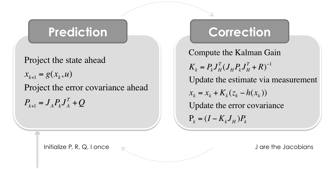
Wikipedia writes: In the extended Kalman filter, the state transition and observation models need not be linear functions of the state but may instead be differentiable functions.
$\boldsymbol{x}_{k} = g(\boldsymbol{x}_{k-1}, \boldsymbol{u}_{k-1}) + \boldsymbol{w}_{k-1}$
$\boldsymbol{z}_{k} = h(\boldsymbol{x}_{k}) + \boldsymbol{v}_{k}$
Where $w_k$ and $v_k$ are the process and observation noises which are both assumed to be zero mean Multivariate Gaussian noises with covariance matrix $Q$ and $R$ respectively.
The function $g$ can be used to compute the predicted state from the previous estimate and similarly the function $h$ can be used to compute the predicted measurement from the predicted state. However, $g$ and $h$ cannot be applied to the covariance directly. Instead a matrix of partial derivatives (the Jacobian matrix) is computed.
At each time step, the Jacobian is evaluated with current predicted states. These matrices can be used in the Kalman filter equations. This process essentially linearizes the non-linear function around the current estimate.
State Vector - Constant Turn Rate and Velocity Vehicle Model (CTRV)
Situation covered: You have a velocity sensor, which measures the vehicle speed ($v$) in heading direction ($\psi$) and a yaw rate sensor ($\dot \psi$) which both have to fused with the position ($x$ & $y$) from a GPS sensor.
Constant Turn Rate, Constant Velocity Model for a vehicle 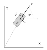
numstates=5 # States
We have different frequency of sensor readings.
dt = 1.0/50.0 # Sample Rate of the Measurements is 50Hz
dtGPS=1.0/10.0 # Sample Rate of GPS is 10Hz
vs, psis, dpsis, dts, xs, ys, lats, lons = symbols('v \psi \dot\psi T x y lat lon')

gs = Matrix([[xs+(vs/dpsis)*(sin(psis+dpsis*dts)-sin(psis))],
             [ys+(vs/dpsis)*(-cos(psis+dpsis*dts)+cos(psis))],
             [psis+dpsis*dts],
             [vs],
             [dpsis]])
state = Matrix([xs,ys,psis,vs,dpsis])
Dynamic Function $g$
This formulas calculate how the state is evolving from one to the next time step
gs
Calculate the Jacobian of the Dynamic function $g$ with respect to the state vector $x$
gs.jacobian(state)
Initial Uncertainty $P_0$
Initialized with $0$ means you are pretty sure where the vehicle starts
P = np.diag([1000.0, 1000.0, 1000.0, 1000.0, 1000.0])
print(P, P.shape)
(array([[ 1000.,     0.,     0.,     0.,     0.],
       [    0.,  1000.,     0.,     0.,     0.],
       [    0.,     0.,  1000.,     0.,     0.],
       [    0.,     0.,     0.,  1000.,     0.],
       [    0.,     0.,     0.,     0.,  1000.]]), (5, 5))
Process Noise Covariance Matrix $Q$
"The state uncertainty model models the disturbances which excite the linear system. Conceptually, it estimates how bad things can get when the system is run open loop for a given period of time." - Kelly, A. (1994). A 3D state space formulation of a navigation Kalman filter for autonomous vehicles, (May). Retrieved from http://oai.dtic.mil/oai/oai?verb=getRecord&metadataPrefix=html&identifier=ADA282853
sGPS     = 0.5*8.8*dt**2  # assume 8.8m/s2 as maximum acceleration, forcing the vehicle
sCourse  = 0.1*dt # assume 0.1rad/s as maximum turn rate for the vehicle
sVelocity= 8.8*dt # assume 8.8m/s2 as maximum acceleration, forcing the vehicle
sYaw     = 1.0*dt # assume 1.0rad/s2 as the maximum turn rate acceleration for the vehicle

Q = np.diag([sGPS**2, sGPS**2, sCourse**2, sVelocity**2, sYaw**2])
print(Q, Q.shape)
(array([[  3.09760000e-06,   0.00000000e+00,   0.00000000e+00,
          0.00000000e+00,   0.00000000e+00],
       [  0.00000000e+00,   3.09760000e-06,   0.00000000e+00,
          0.00000000e+00,   0.00000000e+00],
       [  0.00000000e+00,   0.00000000e+00,   4.00000000e-06,
          0.00000000e+00,   0.00000000e+00],
       [  0.00000000e+00,   0.00000000e+00,   0.00000000e+00,
          3.09760000e-02,   0.00000000e+00],
       [  0.00000000e+00,   0.00000000e+00,   0.00000000e+00,
          0.00000000e+00,   4.00000000e-04]]), (5, 5))
Real Measurements
#path = './../RaspberryPi-CarPC/TinkerDataLogger/DataLogs/2014/'
datafile = '2014-03-26-000-Data.csv'

date, \
time, \
millis, \
ax, \
ay, \
az, \
rollrate, \
pitchrate, \
yawrate, \
roll, \
pitch, \
yaw, \
speed, \
course, \
latitude, \
longitude, \
altitude, \
pdop, \
hdop, \
vdop, \
epe, \
fix, \
satellites_view, \
satellites_used, \
temp = np.loadtxt(datafile, delimiter=',', unpack=True,
                  converters={1: mdates.strpdate2num('%H%M%S%f'),
                              0: mdates.strpdate2num('%y%m%d')},
                  skiprows=1)

print('Read \'%s\' successfully.' % datafile)

# A course of 0° means the Car is traveling north bound
# and 90° means it is traveling east bound.
# In the Calculation following, East is Zero and North is 90°
# We need an offset.
course =(-course+90.0)
Read '2014-03-26-000-Data.csv' successfully.
Measurement Function $h$
Matrix $J_H$ is the Jacobian of the Measurement function $h$ with respect to the state. Function $h$ can be used to compute the predicted measurement from the predicted state.
If a GPS measurement is available, the following function maps the state to the measurement.
hs = Matrix([[xs],
             [ys],
             [vs],
             [dpsis]])
hs
JHs=hs.jacobian(state)
JHs
If no GPS measurement is available, simply set the corresponding values in $J_h$ to zero.
Measurement Noise Covariance $R$
"In practical use, the uncertainty estimates take on the significance of relative weights of state estimates and measurements. So it is not so much important that uncertainty is absolutely correct as it is that it be relatively consistent across all models" - Kelly, A. (1994). A 3D state space formulation of a navigation Kalman filter for autonomous vehicles, (May). Retrieved from http://oai.dtic.mil/oai/oai?verb=getRecord&metadataPrefix=html&identifier=ADA282853
varGPS = 6.0 # Standard Deviation of GPS Measurement
varspeed = 1.0 # Variance of the speed measurement
varyaw = 0.1 # Variance of the yawrate measurement
R = np.matrix([[varGPS**2, 0.0, 0.0, 0.0],
               [0.0, varGPS**2, 0.0, 0.0],
               [0.0, 0.0, varspeed**2, 0.0],
               [0.0, 0.0, 0.0, varyaw**2]])

print(R, R.shape)
(matrix([[  3.60000000e+01,   0.00000000e+00,   0.00000000e+00,
           0.00000000e+00],
        [  0.00000000e+00,   3.60000000e+01,   0.00000000e+00,
           0.00000000e+00],
        [  0.00000000e+00,   0.00000000e+00,   1.00000000e+00,
           0.00000000e+00],
        [  0.00000000e+00,   0.00000000e+00,   0.00000000e+00,
           1.00000000e-02]]), (4, 4))
Identity Matrix
I = np.eye(numstates)
print(I, I.shape)
(array([[ 1.,  0.,  0.,  0.,  0.],
       [ 0.,  1.,  0.,  0.,  0.],
       [ 0.,  0.,  1.,  0.,  0.],
       [ 0.,  0.,  0.,  1.,  0.],
       [ 0.,  0.,  0.,  0.,  1.]]), (5, 5))
Initial State
x = np.matrix([[mx[0], my[0], course[0]/180.0*np.pi, speed[0]/3.6+0.001, yawrate[0]/180.0*np.pi]]).T
print(x, x.shape)

U=float(np.cos(x[2])*x[3])
V=float(np.sin(x[2])*x[3])

plt.quiver(x[0], x[1], U, V)
plt.scatter(float(x[0]), float(x[1]), s=100)
plt.title('Initial Location')
plt.axis('equal')
(matrix([[ 0.        ],
        [ 0.        ],
        [-4.08756111],
        [ 0.67322222],
        [-0.32660346]]), (5, 1))

Extended Kalman Filter
for filterstep in range(m):

    # Time Update (Prediction)
    # ========================
    # Project the state ahead
    # see "Dynamic Matrix"
    if np.abs(yawrate[filterstep])<0.0001: # Driving straight
        x[0] = x[0] + x[3]*dt * np.cos(x[2])
        x[1] = x[1] + x[3]*dt * np.sin(x[2])
        x[2] = x[2]
        x[3] = x[3]
        x[4] = 0.0000001 # avoid numerical issues in Jacobians
        dstate.append(0)
    else: # otherwise
        x[0] = x[0] + (x[3]/x[4]) * (np.sin(x[4]*dt+x[2]) - np.sin(x[2]))
        x[1] = x[1] + (x[3]/x[4]) * (-np.cos(x[4]*dt+x[2])+ np.cos(x[2]))
        x[2] = (x[2] + x[4]*dt + np.pi) % (2.0*np.pi) - np.pi
        x[3] = x[3]
        x[4] = x[4]
        dstate.append(1)

    # Calculate the Jacobian of the Dynamic Matrix A
    # see "Calculate the Jacobian of the Dynamic Matrix with respect to the state vector"
    a13 = float((x[3]/x[4]) * (np.cos(x[4]*dt+x[2]) - np.cos(x[2])))
    a14 = float((1.0/x[4]) * (np.sin(x[4]*dt+x[2]) - np.sin(x[2])))
    a15 = float((dt*x[3]/x[4])*np.cos(x[4]*dt+x[2]) - (x[3]/x[4]**2)*(np.sin(x[4]*dt+x[2]) - np.sin(x[2])))
    a23 = float((x[3]/x[4]) * (np.sin(x[4]*dt+x[2]) - np.sin(x[2])))
    a24 = float((1.0/x[4]) * (-np.cos(x[4]*dt+x[2]) + np.cos(x[2])))
    a25 = float((dt*x[3]/x[4])*np.sin(x[4]*dt+x[2]) - (x[3]/x[4]**2)*(-np.cos(x[4]*dt+x[2]) + np.cos(x[2])))
    JA = np.matrix([[1.0, 0.0, a13, a14, a15],
                    [0.0, 1.0, a23, a24, a25],
                    [0.0, 0.0, 1.0, 0.0, dt],
                    [0.0, 0.0, 0.0, 1.0, 0.0],
                    [0.0, 0.0, 0.0, 0.0, 1.0]])


    # Project the error covariance ahead
    P = JA*P*JA.T + Q

    # Measurement Update (Correction)
    # ===============================
    # Measurement Function
    hx = np.matrix([[float(x[0])],
                    [float(x[1])],
                    [float(x[3])],
                    [float(x[4])]])

    if GPS[filterstep]: # with 10Hz, every 5th step
        JH = np.matrix([[1.0, 0.0, 0.0, 0.0, 0.0],
                        [0.0, 1.0, 0.0, 0.0, 0.0],
                        [0.0, 0.0, 0.0, 1.0, 0.0],
                        [0.0, 0.0, 0.0, 0.0, 1.0]])
    else: # every other step
        JH = np.matrix([[0.0, 0.0, 0.0, 0.0, 0.0],
                        [0.0, 0.0, 0.0, 0.0, 0.0],
                        [0.0, 0.0, 0.0, 1.0, 0.0],
                        [0.0, 0.0, 0.0, 0.0, 1.0]])

    S = JH*P*JH.T + R
    K = (P*JH.T) * np.linalg.inv(S)

    # Update the estimate via
    Z = measurements[:,filterstep].reshape(JH.shape[0],1)
    y = Z - (hx)                         # Innovation or Residual
    x = x + (K*y)

    # Update the error covariance
    P = (I - (K*JH))*P


    # Save states for Plotting
    savestates(x, Z, P, K)
Lets take a look at the filter performance
Uncertainties in $P$
plotP()

State Vector
plotx()

Position x/y
plotxy()

Detailed View
plotxydetails()

Conclusion
As you can see, complicated analytic calculation of the Jacobian Matrices, but it works pretty well.
To use this notebook as a presentation type:
jupyter-nbconvert --to slides Extended-Kalman-Filter-CTRV.ipynb --reveal-prefix=reveal.js --post serve
Questions? @Balzer82