#!/usr/bin/env python
# coding: utf-8
# # Geothermal doublets
#
# In this notebook, we will take a look at geothermal doublets. It will cover the definition of a geothermal doublet installation, explain some _buzzwords_ such as "thermal breakthrough" or "kalina cycle", and show some results of a numerical doublet simulation.
# This simulation is run with SHEMAT-Suite, a numerical code for simulating heat- and mass transfer in a porous medium. The simulations are run on a synthetic model of a graben system over a time of 35 years. That means, we simulate geothermal power production over a lifespan of 35 years.
#
#  # ### Introduction
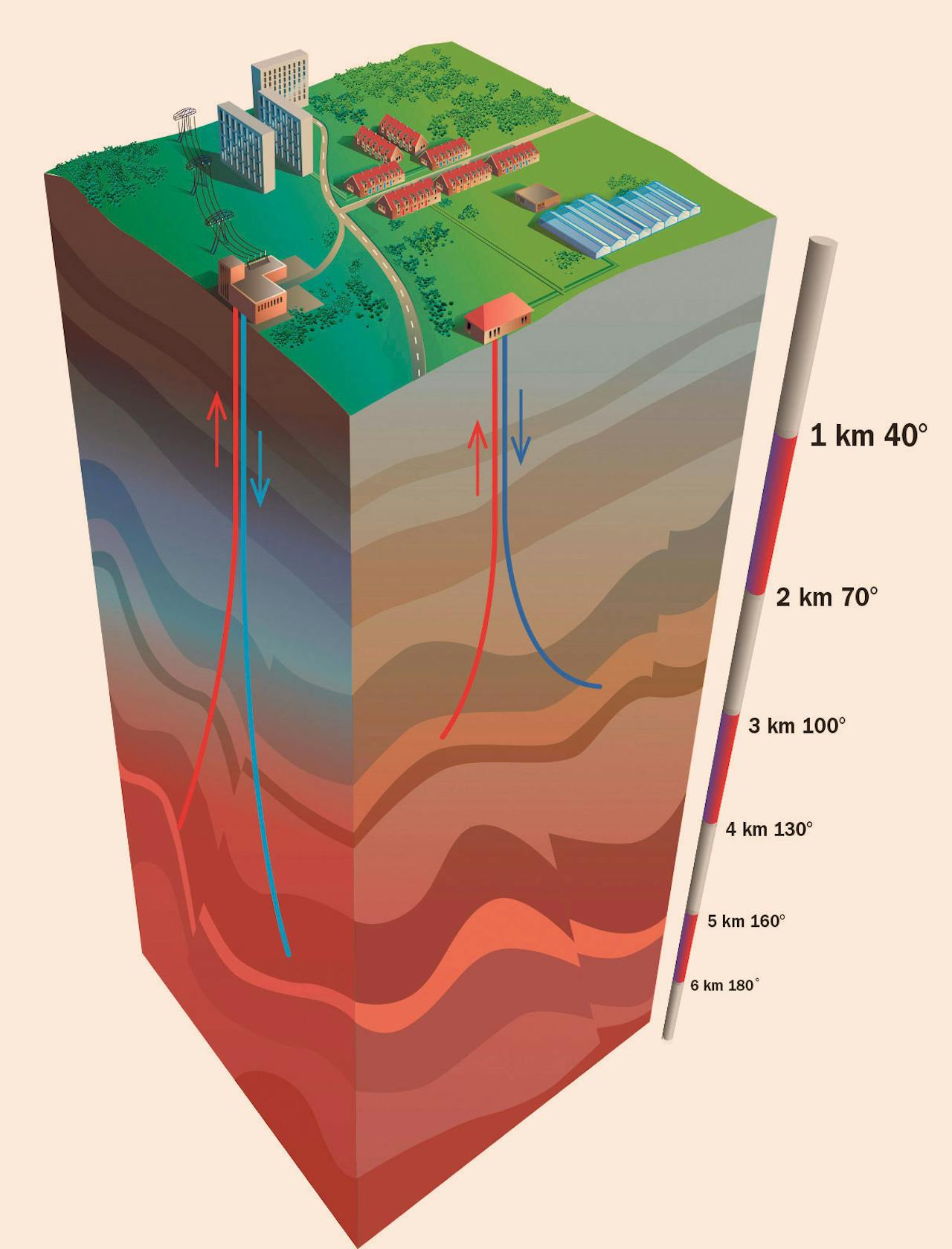
# A geothermal doublet system usually consists of -at least- two boreholes, connected via a surface application installation (such as a powerplant for producing electricity, or an installation for district heating). One geothermal well produces the hot fluid (or steam) from the subsurface. This well is called the producer. The heat of the produced fluid is used accordingly, and the significant cooler fluid is then re-injected in the geothermal reservoir. In the figure to the left, the producing well is marked as a red line, while the injecting well is marked as a blue line, representing the difference in fluid temperature.
#
# If the heat content of the produced "fluid" is large enough, i.e. dry steam is produced, a turbine can be directly operated in one circuit. If the temperatures of the fluide are lower and do not really suffice to operate a turbine directly, a binary cycle is often installed. In such a cycle, the produced fluid heats up a secondary fluid in a heat-exchanger. This secondary fluid has a significantly lower boiling point, an can thus be used to operate a turbine instead. Such a system is often called a [Kalina installation](https://en.wikipedia.org/wiki/Kalina_cycle), where the secondary fluid is a mixture of water and ammonia.
#
# Operating such a system over a prolonged time will eventually cause a decrease in production temperature, as the cooling front of the re-injected water reaches the producing borehole. The point in time, where production temperature starts to decrease significantly is called a _thermal breakthrough_. In the results of a simplified doublet simulation, which we study in this notebook, we will also look for a thermal breakthrough.
#
# ### Introduction
# A geothermal doublet system usually consists of -at least- two boreholes, connected via a surface application installation (such as a powerplant for producing electricity, or an installation for district heating). One geothermal well produces the hot fluid (or steam) from the subsurface. This well is called the producer. The heat of the produced fluid is used accordingly, and the significant cooler fluid is then re-injected in the geothermal reservoir. In the figure to the left, the producing well is marked as a red line, while the injecting well is marked as a blue line, representing the difference in fluid temperature.
#
# If the heat content of the produced "fluid" is large enough, i.e. dry steam is produced, a turbine can be directly operated in one circuit. If the temperatures of the fluide are lower and do not really suffice to operate a turbine directly, a binary cycle is often installed. In such a cycle, the produced fluid heats up a secondary fluid in a heat-exchanger. This secondary fluid has a significantly lower boiling point, an can thus be used to operate a turbine instead. Such a system is often called a [Kalina installation](https://en.wikipedia.org/wiki/Kalina_cycle), where the secondary fluid is a mixture of water and ammonia.
#
# Operating such a system over a prolonged time will eventually cause a decrease in production temperature, as the cooling front of the re-injected water reaches the producing borehole. The point in time, where production temperature starts to decrease significantly is called a _thermal breakthrough_. In the results of a simplified doublet simulation, which we study in this notebook, we will also look for a thermal breakthrough.
#
[Image source](https://images.fd.nl/archive/89002_def-tno-geothermie.jpg?fit=crop&crop=faces&auto=format%2Ccompress&q=45&w=1280)
#
# In[1]:
# necessary libraries
import h5py
import pandas as pd
import numpy as np
import matplotlib.pyplot as plt
get_ipython().run_line_magic('matplotlib', 'inline')
# for improving plot aesthetics
import seaborn as sns
sns.set_style('ticks')
sns.set_context('poster')
# ## 3D reservoir model
# For assessing this (rather cold) geothermal system, we simulate the heat- and mass transfer in a synthetic, three dimensional model. The model consists of 4 geological units:
# * Basement
# * Bottom Unit
# * Reservoir Unit
# * Top Unit
#
# The reservoir Unit is a geological body with a high primary porosity and permeability, which enables a natural darcy flow, and also shows advective heat transport by convection. Convection increases the geothermal potential of a system, as hot fluids are flowing upwards due to lower density, cooling down, and descending again. Kind of like [lava lamps](https://lavalamp.com/wp-content/uploads/2016/08/6825_1500x2000.jpg), which were popular back in the days.
# In the plot below, we see a vertical cross-section of the model in x-direction (let's say an East-West cross-section). On the left, you can see the geological units with annotations, on the right the natural temperature field. There, we can already see strongly bent isothermes, which are caused by an interplay of differences in thermal conductivity of the geological units, and advective heat transport.
# For assessing, which of those processes, i.e. conductive vs. advective heat transport, we could perform a peclet number analysis (there will also be a notebook on peclet number analysis in this repository). For the moment, it is sufficient to state, that both processes are present in this model.
# In[12]:
# 3D model file
mod = h5py.File('data/Input_f_final.h5')
x = mod['x'][0,0,:]
y = mod['y'][0,:,0]
z = mod['z'][:,0,0]
t = mod['temp'][:,:,:]
ui = mod['uindex'][:,:,:]
vx = mod['vx'][:,:,:]
vy = mod['vy'][:,:,:]
vz = mod['vz'][:,:,:]
mod.close()
# doublet position
prod = np.array([74, 29, 15])
inj = np.array([41, 29, 15])
# plot routine
cs = 29 # cross -section position
fig, axs = plt.subplots(1, 2, figsize=[15,5], sharey=True, sharex=True)
ax1 = axs[0].contourf(x, z-2000, ui[:,cs,:], 4, cmap= 'viridis') # geological units
ax2 = axs[1].contourf(x, z-2000, t[:,cs,:], cmap='viridis') # temperature
# plot doublet positions
axs[0].plot(prod[0]*20, (prod[2]*50-2000), 'ro')
axs[0].plot(inj[0]*20, (inj[2]*50-2000), 'bo')
axs[1].plot(prod[0]*20, (prod[2]*50-2000), 'ro')
axs[1].plot(inj[0]*20, (inj[2]*50-2000), 'bo')
axs[0].vlines(prod[0]*20, prod[2]*50-2000,0)
axs[0].vlines(inj[0]*20, inj[2]*50-2000,0)
axs[1].vlines(prod[0]*20, prod[2]*50-2000,0)
axs[1].vlines(inj[0]*20, inj[2]*50-2000,0)
#axs[1].streamplot(x, z-2000, vx[:,cs,:], vz[:,cs,:], density=[1, .5], color='white')
# axes arguments
axs[0].set_ylabel('model height [m]')
axs[0].set_xlabel('y [m]')
axs[1].set_xlabel('y [m]')
# annotations
axs[0].text(100, -1850, 'Basement', color=[.9,.9,.9])
axs[0].text(100, -1400, 'Reservoir', color=[.9,.9,.9])
axs[0].text(100, -950, 'Thermal blanket', color=[.9,.9,.9])
axs[0].text(100, -280, 'Overburden', color=[.3,.3,.3])
# colormap
fig.subplots_adjust(right=0.8)
cbar_ax = fig.add_axes([1., 0.21, 0.03, 0.7])
fig.colorbar(ax2, cax=cbar_ax, label= 'T °C')
# layout option
plt.tight_layout()
fig.savefig("doublet_example.png", dpi=400, bbox_inches='tight')
# Temperatures in the model range from 10 °C to 80 °C. These temperatures are not sufficiently high for direct geothermal electricity generation, but potentially appropriate for a binary system or a system for direct-heat usage. One interesting characteristic of this model is the convective heat transport. Next to temperature, you can see streamlines in the right plot above. These lines visualise the flow field (and may be used to visualise every vector field you have). Essentially, with a stable convective system, producing from upwelling areas (where hot water rises due to its relatively lower density) is good, as higher temperatures are encountered at shallower depths.
# Despite the low temperature range we simulated, the following assessment can generally be applied to doublet systems, regardless of the produced temperatures. Speaking of produced temperatures, in the model above, we implemented a doublet system, where the flow rate (i.e. the rate at which the pump operates) is varied.
# Below, we plot the temperature at the producing borehole with time.
# In[3]:
# load monitoring files
pr_50L = pd.read_csv('data/doublet_50ls.csv', comment='%')
pr_75L = pd.read_csv('data/doublet_75ls.csv', comment='%')
pr_100L = pd.read_csv('data/doublet_100ls.csv', comment='%')
fig = plt.figure(figsize=[12,6])
p50 = plt.plot(pr_50L['time'], pr_50L['temp'], '--', label='50 L s$^{-1}$')
p75 = plt.plot(pr_75L['time'], pr_75L['temp'], '--', label='75 L s$^{-1}$')
p100 = plt.plot(pr_100L['time'], pr_100L['temp'], '--', label='100 L s$^{-1}$')
plt.legend()
plt.ylabel('Temperature [°C]')
plt.xlabel('time [a]')
fig.tight_layout()
# Over the simulated time of 35 years, you can see the temperatures produced from the production borehole (red circle in the cross sections above). Note how the temperatures rapidly decrease at the beginning of the simulation. As we implement the doublet as a boundary condition (i.e. a source/sink term), the system has to react to the newly applied boundary conditions. However, after around 1 year, the system is re-equilibrated and produced temperatures can be assessed.
# One thing of interest for example is the thermal breakthrough of a system, the point in time, when the temperature signal of the cold, re-injected water reaches the production borehole.
# Subsurface parameters, such as hydraulic head distribution or reservoir permeability affect the timing of a thermal breakthrough. But it is also influenced by operation parameters, e.g. pumping rate and injection temperature. In the plot above, we model the same doublet layout with three different pumping rates, and we see that 100 l s$^{-1}$ correlate to an earlier thermal breakthrough, when compared to the other pumping rates (75 l s$^{-1}$ and 50 l s$^{-1}$).
# While knowledge about the development of the production temperature over time is important, other parameters, such as the transient change in obtained thermal power are equally or even more interesting. Thermal power of a geothermal doublet can be calculated using the following equation:
#
# $$ P_{th} = Q (\rho c_p)_w (T_{pr} - T_{in}) $$
#
# where P$_{th}$ is the thermal power in W, Q the pumping rate in m³ s$^{-1}$ ($\rho c_p)_w$) the thermal capacity of water in W m$^{-3}$ K$^{-1}$ and (T$_{pr}$ - T$_{in}$) the difference between production temperature and injection temperature (in K). Let's have a look at the thermal power produced by the doublet with three different pumping rates.
# In[4]:
def therm_pow(Q, rhocp, Tin, Tpr):
"""
A short function for calculating the thermal power
Q - scalar, flow rate in m³/s
rhocp - scalar, thermal capacity of water in W/(m³K)
Tin - scaler, re-injection temperature of the water in °C
Tpr - vector, production temperature of the water in °C
"""
return Q*rhocp*(Tpr-Tin)
# In[5]:
# parameter
Q = np.array([0.05, 0.075, 0.1]) # 50 L/s, 75 L/s, 100 L/s
rhocp = 988 * 4180 # density and specific heat capacity of water at a temperature of about 50 °C
Tin = 30 # injection temeprature in °C
# calculate thermal power
thp50 = therm_pow(Q[0], rhocp, Tin, pr_50L['temp'])
thp75 = therm_pow(Q[1], rhocp, Tin, pr_75L['temp'])
thp100 = therm_pow(Q[2], rhocp, Tin, pr_100L['temp'])
# In[6]:
# plot
d2MW = 1e6 # use for calculating in MW
fig = plt.figure(figsize=[12,6])
p50 = plt.plot(pr_50L['time'], thp50/d2MW, '--', label='50 L s$^{-1}$')
p75 = plt.plot(pr_75L['time'], thp75/d2MW, '--', label='75 L s$^{-1}$')
p100 = plt.plot(pr_100L['time'], thp100/d2MW, '--', label='100 L s$^{-1}$')
plt.legend()
plt.ylabel('therm. power [MW]')
plt.xlabel('time [a]')
fig.tight_layout()
# Logically, the highest flow rate yields the highest thermal power. The timing of thermal breakthrough and its intensity are however visible, as the produced thermal power with a flow rate of 100 L s$^{-1}$ declines significantly stronger than lower flow rates. In this scenario, this may not cause a problem.
# In the exercise course, we will assess a different reservoir system where the significantly different evolution of production temperatures depending on the chosen pumping rate will visualise the importance of monitoring the reservoir and the production temperatures.